CI Functions for Effect Size d

In Confidence Interval for Effect Size and Power, we show how to calculate a confidence interval for Cohen’s effect size based on a confidence interval for the noncentrality parameter using data from a t-test. On this webpage, we show how to calculate confidence intervals for the effect size directly from the sample data. We will also show how to use Real Statistics functions to quickly calculate such confidence intervals.

One Sample Test

We start by describing how to manually calculate the confidence interval for a one-sample Cohen’s d effect size using the confidence interval of the noncentrality parameter.

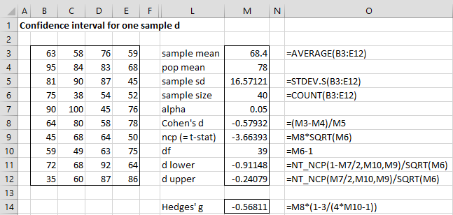
Example 1: Find a 95% confidence interval for Cohen’s d for the test from Example 4 of One Sample t Test. This is also Example 1 of Confidence Interval for Effect Size and Power.

We repeat the data on the left side of Figure 1, with the results shown on the right side of the figure.

Figure 1 – Calculating 95% confidence interval for the effect size

Note that the (-.91148, -.024079) confidence interval is quite similar to the 95% confidence interval (-.91421, -.24443) found in One-sample Effect Size using the Hedges and Olkin approach. On that webpage, we also introduced the T_EFFECT1 and TT_EFFECT1 array functions. We now describe the complete format of these functions.

Worksheet Functions

Real Statistics Functions: The Real Statistics Resource Pack contains the following array functions.

T_EFFECT1(m, s, n, lab, alpha, iter, iter0, prec) = column array with the values Cohen’s d, Hedges’ g, and the lower and upper confidence interval limits for d based on a one-sample t-test for data with mean m, standard deviation s and sample size n.

TT_EFFECT1(R1, hyp, lab, alpha, iter, iter0, prec) = T_EFFECT1(m, s, n, lab, alpha, iter, iter0, prec) where m = AVERAGE(R1) – hyp, s = STEV.S(R1) and n = COUNT(R1).

alpha is the significance level (default .05). If lab = TRUE (default FALSE) then an extra column of labels is appended to the output. hyp = the hypothetical (i.e. population) mean (default 0).

The last three arguments are as for the NT_NCP function (see Noncentral t Distribution), except that if iter = 0 then the Hedges and Olkin estimate of the confidence interval is employed (iter0 and prec are not used), while if iter > 0 (default 1000) then the estimate of the confidence interval described above based on the noncentrality parameter is used. In this case, iter, iter0, and prec are as for the NT_NCP function (see Noncentral t Distribution).

For Example 1, the output from =TT_EFFECT1(A5:D14, 78, TRUE) is formatted as shown in Figure 2 of One-Sample Effect Size, except that now the values are those shown in cells M8, M14, M11, and M12 from Figure 1 above.

Two Independent Sample Test

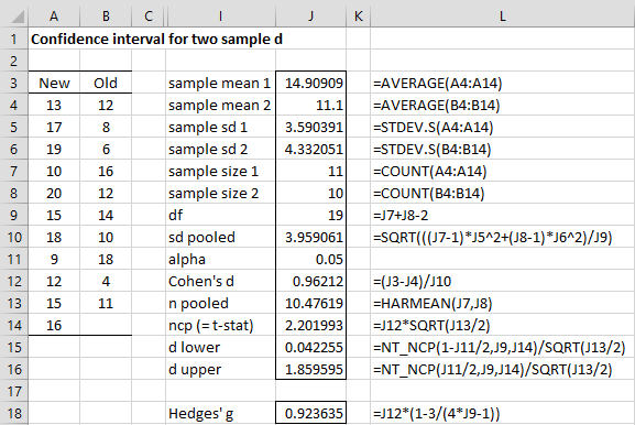
Example 2: Find the 95% confidence interval of the effect size for Example 1 of Two-Sample t-Test with Equal Variances, repeating the analysis shown in Figure 4 of Two-Sample Effect Size using the noncentrality approach.

We repeat the data on the left side of Figure 2, with the results shown on the right side of the figure.

Figure 2 – Confidence interval for two sample d effect

Note that the (.042255, 1.859595) confidence interval is quite similar to the 95% confidence interval (-.91421, -.24443) we found Two-Sample Effect Size using the Hedges and Olkin approach. On that web page, we also introduced the T_EFFECT2 and TT_EFFECT2 array functions. We now describe the complete format of these functions.

Worksheet Functions

Real Statistics Functions: The Real Statistics Resource Pack contains the following array functions.

T_EFFECT2(m1, s1, n1, m2, s2, n2, lab, alpha, iter, iter0, prec) = column array with the values Cohen’s d, Hedges’ g and the lower and upper confidence interval limits for d based on a two independent sample t-test for sample 1 with mean m1, standard deviation s1, and sample size n1, and sample 2 with mean m2, standard deviation s2  and sample size n2.

TT_EFFECT2(R1, R2, lab, alpha,  iter, iter0, prec) = T_EFFECT2(m1, s1, n1, m2, s2, n2, lab, alpha, iter, iter0, prec) where m1 = AVERAGE(R1), s1 = STEV.S(R1), n1 = COUNT(R1), m2 = AVERAGE(R2), s2 = STEV.S(R2) and n2 = COUNT(R2).

alpha, iter, iter0, prec are as described above for the T_EFFECT1 and TT_EFFECT1 functions.

For Example 2, the output from the array worksheet formula =TT_EFFECT1(A4:A14,TRUE) is formatted as shown in Figure 2 of Two-Sample Effect Size, except that now the values are those shown in cells J12, J18, J15 and J16 of Figure 2 above.

Paired Sample Test

We can create a confidence interval for the d effect size using the approach for a one-sample t-test based on the sample differences).

As described in Paired t-Test, we can create a confidence interval for the d_z effect size using the approach for a one-sample t-test (based on the sample differences). Although d_z is the effect size used to calculate statistical power for the paired t-test, in many other situations, the preferred effect size statistic is d_av

where

We now show how to create confidence intervals for this measure of effect size.

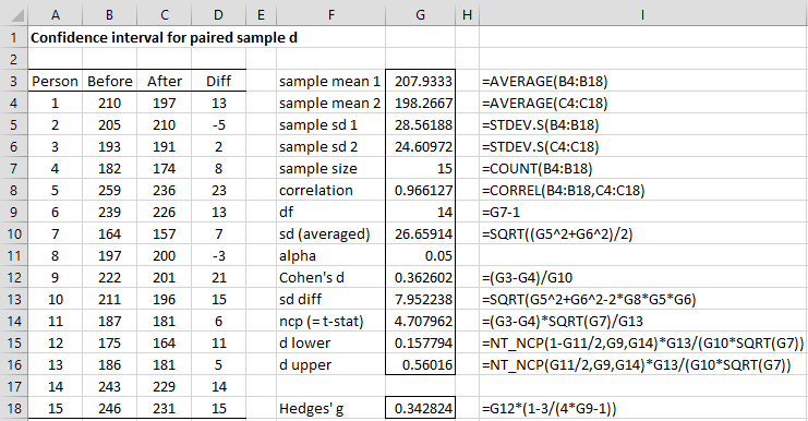
Example 3: Find the 95% confidence interval of the effect size d_av for Example 1 of Paired t Test.

The analysis is shown in Figure 3.

Figure 3 – Confidence for effect size in paired samples test

We see that d_av = .3626 with a 95% confidence interval of (.1578, .5602) and Hedges’ g_av = .3428. We can get the same results by using the following Real Statistics functions.

Worksheet Functions

Real Statistics Functions: The Real Statistics Resource Pack provides the following array functions.

T_EFFECT2P(m1, m2, s1, s2, r, n, lab, alpha, iter, iter0, prec) = column array with the values Cohen’s d_av, Hedges’ g_av and the lower and upper confidence interval limits for d_av based on a paired sample t-test for sample 1 with mean m1, standard deviation s1  and sample size n, and sample 2 with mean m2, standard deviation s2 and sample size n. r = the correlation coefficient between samples 1 and 2.

TT_EFFECT2P(R1, R2, lab, alpha, iter, iter0, prec) = T_EFFECT2P(m1, m2, s1, s2, r, n, lab, alpha, iter, iter0, prec) where m1 = AVERAGE(R1), s1 = STEV.S(R1), n = COUNT(R1) = COUNT(R2), m2 = AVERAGE(R2), s2 = STEV.S(R2) and r = CORREL(R1, R2).

alpha is the significance level (default .05). If lab = TRUE (default FALSE) then an extra column of labels is appended to the output.

alpha, iter, iter0, prec are as described above for T_EFFECT1 and TT_EFFECT1, except iter must take a positive integer (no Hedges-Olkin version is supported).

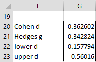
Referring to Figure 3, the array formulas =T_EFFECT2P(G3, G4, G5, G6, G8, G7, TRUE) and =TT_EFFECT2P(B4:B18, C4:C18, TRUE) result in the output shown in Figure 4.

Figure 4 – 95% confidence interval for d_av effect size

References

Hedges, L. V. and Olkin, I. (1985) Statistical methods for meta-analysis. Academic Press
https://www.researchgate.net/publication/216811655_Statistical_Methods_in_Meta-Analysis

Enzmann, D. (2015) Notes on Effect Size Measures for the Difference of Means From Two Independent Groups: The Case of Cohen’s d and Hedges’ g
Available through Researchgate

SAGE Publications (2019) t-tests: one-sample, two-independent-sample, and related-samples design.
https://us.sagepub.com/sites/default/files/upm-assets/98047_book_item_98047.pdf

Lakens, D. (2013) Calculating and reporting effect sizes to facilitate cumulative science: a practical primer for t-tests and ANOVAs. Frontiers in Psychology.
https://www.frontiersin.org/articles/10.3389/fpsyg.2013.00863/full

Ellis, P. D. (2010) The essential guide to effect size. Cambridge University Press.
http://rauterberg.employee.id.tue.nl/lecturenotes/DBB150/references/Ellis-2010%20Essential%20Guide%20to%20Effect%20Sizes.pdf

Howell, D. C. (2010) Confidence intervals on effect size
https://www.uvm.edu/~statdhtx/methods8/Supplements/MISC/Confidence%20Intervals%20on%20Effect%20Size.pdf