Objective
As described in Null Hypothesis Testing, beta (β) is the acceptable level of type II error, i.e. the probability that the null hypothesis is not rejected even though it is false. Statistical power is 1 – β, and so represents the probability that the null hypothesis is correctly rejected (when it is false), or in other words it is the probability that an effect is correctly identified.
We now show how to estimate the power of a statistical test and the related problem of determining the minimum sample size for a test to achieve a desired power. We look at the following situations:
- One-sample, one-tailed test – this webpage
- One-sample, two-tailed test
- Two-sample test
- Real Statistics capabilities
Power Curve
Example 1: Suppose bolts are being manufactured using a process for which it is known that the length of the bolts follows a normal distribution with a standard deviation of 12 mm. The manufacturer wants to check that the mean length of their bolts is at least 60 mm, and so takes a sample of 110 bolts and uses a one-tail test with α = .05 (i.e. H0: µ ≤ 60). What is the probability of a type II error if the measured mean length is 62.5?
Since n = 110 and σ = 12, the standard error = = 1.144. Let x = the length of the bolt. The null hypothesis is rejected provided the sample mean is greater than the critical value of x, which is NORM.INV(1 – α, μ, s.e.) = NORM.INV(.95, 60, 1.144) = 61.88.
Now suppose that the actual mean is 62.5. The situation is illustrated in Figure 1, where the curve on the left represents the normal curve being tested (based on the null hypothesis) with a mean of μ0 = 60, and the normal curve on the right represents the distribution with a mean of μ1 = 62.5.
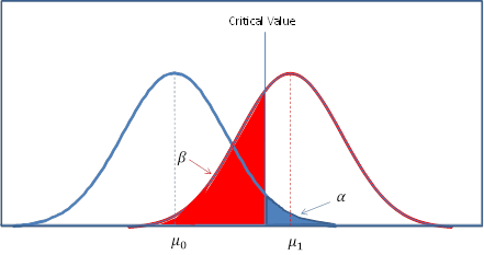 Figure 1 – Statistical power
We have β = NORM.DIST(61.88,62.5,1.144,TRUE) = .295, and so power = 1 – β = .705.
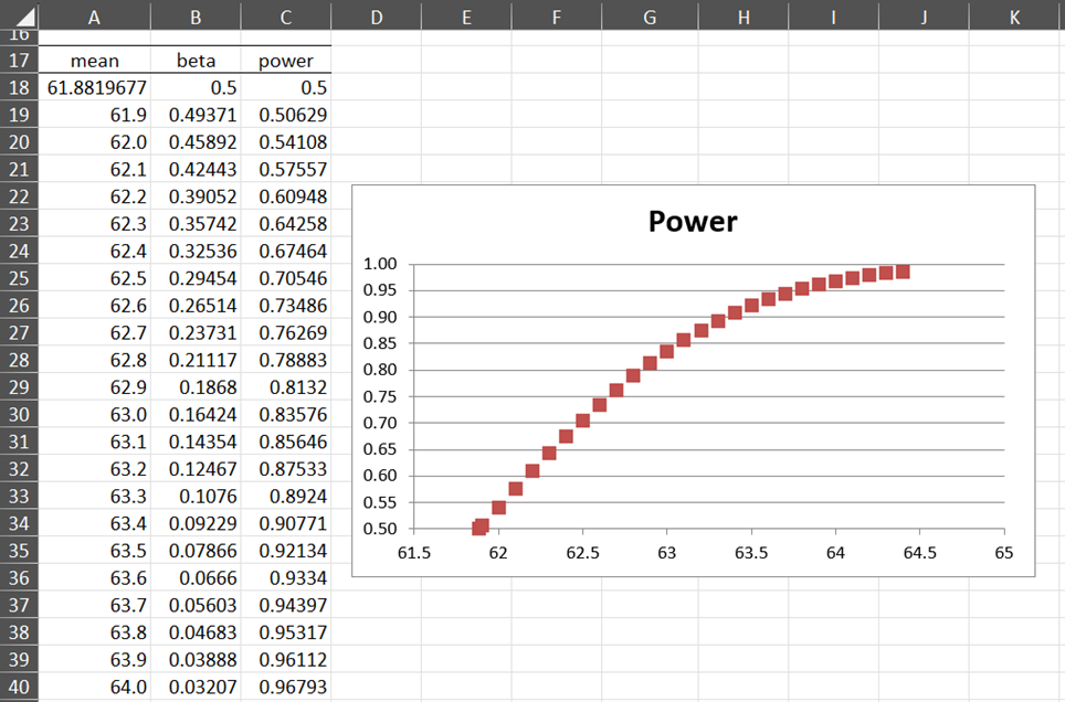
We can repeat this calculation for values of μ1 ≥ 62.5 to obtain the table and graph of the power values in Figure 2.
Figure 2 – Power curve for Example 1
Example
Example 2: For the data in Example 1, answer the following questions:
- What is the power of the test for detecting a standardized effect of size .2?
- Which the smallest effect size (and mean) that can be detected with power .80?
- What sample size is required to detect an effect of size of .2 with power .80?
Using Goal Seek
Determine power
a) As described in Standardized Effect Size, we use the following measure of effect size:
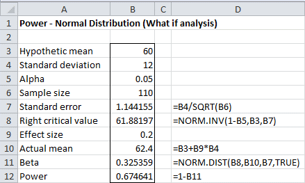
Assuming μ1 ≥ 60, we see that μ1= 60 + (.2)(12) = 62.4. As in Example 1, we see that
β = P(x̄ ≤ xcrit | μ = 62.4) = NORM.DIST(61.88, 62.4, 1.144, TRUE) = .325
and so power = 1 – β = 67.5%.
We summarize these calculations in the following worksheet:
Figure 3 – Determining power based on effect and sample size
Determine effect size
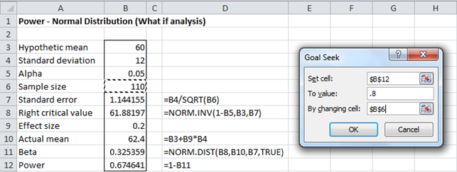
b) We utilize Excel’s Goal Seek capability to answer the second question. Referring to the worksheet in Figure 3, we now select Data > Forecast| What-If Analysis... > Goal Seek (or Data > Data Tools | What-If Analysis.. > Goal Seek for versions of Excel prior to Excel 2016). In the dialog box that appears enter the values shown in Figure 4.
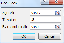
Figure 4 – Goal Seek dialog box
Here, we are requesting that Excel find the value of cell B9 (the effect size) that produces a value of .8 for cell B12 (the power). The Set cell field in the dialog box must point to a cell which contains a formula. The To value field must contain a numeric value and the By changing cell field must point to a cell which contains a value (possibly blank) and not a formula. After clicking on the OK button, a Goal Seek Status dialog box appears and the worksheet from Figure 3 changes to that shown in Figure 5.
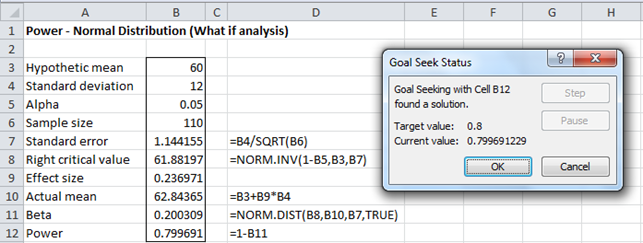
Figure 5 – Determining detectable effect size for specified power
Note that the values of some of cells have changed to the values necessary to obtain the target power of .80. In particular, we see that the Effect size (cell B9) now contains the value 0.23691 and the Actual mean contains the value 62.84. You must click on the OK button in the Goal Seek Status box to lock in these new values (or Cancel to return to the original worksheet values).
Thus, the smallest effect size that can be detected with power of 80% is .23691, with a corresponding mean of 62.84.
Determine sample size
c) We again use Excel’s Goal Seek capability to answer the third question. Referring to the worksheet in Figure 3 (making sure to reset the effect size in cell B9 to .2), we now enter the values shown in the dialog box that appears on the right side of Figure 6.
Figure 6 – Using Goal Seek to determine minimum sample size
After clicking on the OK button, the worksheet changes to that shown in Figure 7.
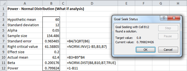
Figure 7 – Sample size requirement for Example 2
In particular, note that the sample size value in cell B6 changes to 154.486. The required sample size is therefore 155 (rounding up).
Alternative Approach
We next show how to use the standard normal distribution to accomplish the same power calculations. We can use this approach for both one-tailed and two-tailed tests.
Determine statistical power
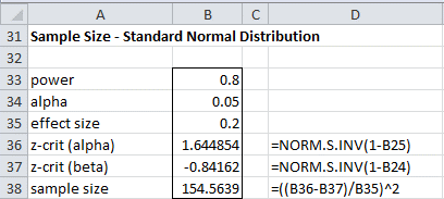
As we see from Figure 3
and so
It now follows that
Also from Figure 3, we see that
where Φ(z) = NORM.S.DIST(z, TRUE), i.e. the cdf of the standard normal distribution, and d is Cohen’s effect size (see Standardized Effect Size). The value d√n is called the non-centrality parameter.
Thus, we now have an alternative way of addressing Example 2 (a), as shown in Figure 8.
Figure 8 – Determining power for a given effect size
Determine effect size and sample size
As we saw above
Solving for beta, we get
Solving for d, we get
where zβ = NORM.S.INV(β). Finally, solving for n, we get
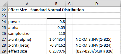
These formulas provide an alternative way of addressing Example 2 (b) and (c), as shown in Figures 9 and 10. Note that this approach doesn’t require the Goal Seek capability.
Figure 9 – Determining detectable effect size for specified power
Figure 10 – Determining sample size for a given effect size
Examples Workbook
Click here to download the Excel workbook with the examples described on this webpage.
References
Faul, F., Erdfelder, E., Buchner, A., & Lang, A. G. (2009). Statistical power analyses using G*Power 3.1: Tests for correlation and regression analyses. Behavior Research Methods, 41, 1149-1160.
http://link.springer.com/article/10.3758/BRM.41.4.1149
STAT (2015) Power and sample size reference manual, release 13
http://www.stata.com/manuals13/pss.pdf
Bhandari, P. (2021) Statistical power and why it matters | a simple introduction
https://www.scribbr.com/statistics/statistical-power/


Hello Charles,
I would like to perform analysis as shown in figure 3, but I wish to look for an effect size in the negative direction (mu1 less than mu0). How should I proceed? I’m sorry if you’ve already answered this question, but I looked through the comments and I’m still not sure how to go about it.
Paul,
It doesn’t matter which direction is required, the calculation is the same. Of course, the direction you are testing for is towards the alternative hypothesis (which is where power makes sense).
You can use the following Real Statistics tool to calculate power.
https://www.real-statistics.com/hypothesis-testing/real-statistics-power-data-analysis-tool/
Charles
Dear Charles
Hope you are doing well, could you please clarify the followings.
In the real scenario, we are using multi-stage sampling (for example, first stage Probability Proportional to Size techniques and the second stage using cluster sampling techniques). So in many cases, each element of the sample does not have the same overall probability of selection (unless select equal number of elements is chosen in each cluster at the second stage of sample selection).
My question, if it is a case (each element of the sample does not have the same overall probability of selection)
• Shall we do the Z or t-test for this selected sample?
My second query
In the real survey, we are facing difficulties to estimate population parameter confidence interval when using multi-stage sampling (for example, first stage Probability Proportional to Size techniques and second stage using cluster sampling techniques) as facing difficulties to calculate the standard error. Could you please to suggest or circulate good guide that describes the equations for calculating estimator (sample mean, sample proportion, sample total) and its variances in the multi-stage sampling (example, PPS first stage and cluster/stratifies in the second stage)
To overcome this problem shall we use the self-weighing technique?
Whenever possible, clusters should be chosen with probability-proportional-to-size in sample surveys at the first stage.
A second is that, if an equal number of elements is chosen in each cluster at the second stage of sample selection, the end result will be a sample in which each element has the same overall probability of selection, or is self-weighting.
Then we can estimate population parameter and its variance using the same technique of simple random sampling without replacement as each element of the sample is having equal overall probability of selection.
In this case, shall we use Z or t-test for this sample?
I haven’t looked into these issues yet. I assume that whether you use the z test or t test, the main issue is how to estimate the variance so that you can estimate the effect size desired. In any case, the following article may be helpful.
http://ocw.jhsph.edu/courses/StatMethodsForSampleSurveys/PDFs/Lecture5.pdf
Charles
Dear Sir
Thank you so much.
Kind regards
V.Valavan
Dear Sir
Hope you are doing well, I want to ask a clarification when your time permit, please throw some light on it.
Which is the best way to estimate the (population) parameter?
1. Calculate the required sample size by defining Z-score (95%, 1-96), error (example 0, 03), and p (say .5 for maximum sample size) then estimate the sample statistic (example sample proportion). Then we say the calculated sample proportion is an unbiased estimator of the population proportion and 95% confidence the population proportion lies within plus or minus 0.03 (this value was used for calculating sample size) of the sample proportion. That is,
p- 0.03=< P <= p + 0.03
Or
We take a small sample (not calculate sample size statistically, say 40) due to limitation but using sampling techniques (srs, cluster or ..) while selecting a sample, then calculate the sample proportion after that and its variance (using statistical techniques). Finally, we say population proportion-P lies between p + – Z SE(p). That is,
p- Z[SE(p)] =< P <= p + Z [SE(p)]
Please clarify it, when your time permits.
Valavan,
Although it depends on exactly what hypothesis you are trying to test and how feasible it is to obtain a sufficiently large sample, the first approach is usually better.
Charles
Thank you very much, sir
Charles,
“Figure 1–Statistical power” helped me understand type II error for a 1-tail comparison. This calculation requires an alternative distribution with a mean of mu1.
I know the type II error (beta) can be calculated for a 2-tail comparison, but I don’t understand what it means. Is the null distribution compared to two alternative distributions having means of mu1 and -mu1? I would really appreciate an illustrated example of finding beta for a 2-tail t-test analysis.
Hi Dave,
It is difficult to understand these concepts without looking at specific examples. I suggest that you look at
https://real-statistics.com/sampling-distributions/statistical-power-sample/
https://real-statistics.com/students-t-distribution/statistical-power-of-the-t-tests/
Charles
Thanks for the links. I had to learn how to use the noncentral t distribution function NT_DIST, but I think I can visualize the process now. The way I would describe beta for a 2-tail analysis is the area of the alternative t distribution INSIDE the right and left t critical values obtained from the null t distribution.
Thanks for this.
I think for figure 2, the values of μ1 are from “61.8819676776998 to 64.4” rather than “μ1 ≥ 62.5”. I found this confusing until I realised this..
Rob,
Sorry about the confusion. I wanted to show the power curve starting from .50. This is clearly labelled in Figure 2.
Charles
Hi Charles,
I have a more philosipoical question.
As I understand the “standardize effect size” concept, it takes the change you want to identify and normalized to a measure of ability to be detectable.
I don’t understand why is it interesting?
you wrote “Since it is standardized we can compare the effects across different studies with different variables” can you please give an interesting example?
In your example you expect the length of the bolt to be 60mm , and maybe 60±1 is okay and more or less can’t be sold in the shops. or 60±1.66%
So I’m interested what is the power of the test to identify bolts longer than 61 or shorter than 59. not what is the power of the test to identify cohen’s d=0.2
maybe in your example, you changed machine and now you compare the effect on the average length to the effect on the average diameter???
I hope it is okay I’m asking many questions.
Thanks a lot,
Oren
Oren,
1. The effect size is interesting since you want to quantify the effect (small, large, etc.). E.g. if you are measuring the effectiveness of a new drug for curing a type of cancer, you prefer a bigger effect size than that of the currently used drug or a placebo.
When you do statistical analysis often you are looking to see whether an effect is statistically significant (using the p-value). This just means that the effect size is different from zero (or some other predesignated value), not whether you should care about the effect. Also as the sample size gets larger and larger it is very likely that you will see a significant result — even if the effect size is very small.
2. You need to look at the literature in your field to see interesting examples of comparisons of effect sizes across different studies, but the example I gave above indicates what to look for. If the effect size of the currently used treatment over a placebo is .30 and your new treatment has an effect size of .70 over a placebo, this will be interesting.
3. Bolt size (i.e. mean bolt size) can easily be mapped into an effect size
Charles
Hello Charles,
why is in the first formula, when you calculate lenght for alpha=0,05 used SEM and not SD? According normal distribution, the 95% of data are within mean +- 2 SD, so it should be =norm.inv(0.95,60,12).
I am not exactly sure which is the first formula that you are referring to, but if it is the effect size formula, then Cohen’s d uses the standard deviation and not the standard error. d does not depend on the sample size.
Charles
I was speaking about example 1, when you calculate alpha a and beta, you used SE =1.44 not SD =12
Vendula,
Yes, for this problem, the appropriate value for the standard deviation for a sample of size 110 is 1.44, which is the standard error for the sample. 12 represents the standard deviation of the population.
Charles
Hi Charles,
I’m interested in how you’d compute beta for observed values that aren’t greater than Xcrit.
For example, if the observed value was 60.5 (less than Xcrit) would the beta be equal to NORMDIST(61.88, 60.5, 1.144, TRUE) = 0.886148, and the beta would be higher the smaller the number gets.
Also, if you were doing a right tail test and the observed value was less than Xcrit, such as NORMDIST(58.12, 58, 1.144, TRUE) = 0.5412.
Thanks
Hello,
If I have a sample with a mean of 1000 and SEM (standar error) of 60 and other sample with a mean of 800 and SEM – 70, how would I calculate the statistical power between these two samples?
Thank you
If you could explain how to to solve it using both excel and spss it would be perfect!! thank you
I don’t use SPSS and so won’t comment about SPSS. See response to your other comment regarding Excel.
Charles
You also need to know the sample size. See the following webpage for details:
Power of t test
Charles
Hello Charles,
I need assistance with how to plug in the numbers for the Statistical Power and Sample Size option. I will be running a logistic regression. I have all the data, but am unsure as to what I input.
Any insight you have would be great! Thank you.
Angela, sorry but the Statistical Power and Sample Size data analysis tool supports linear regression but does not yet support logistic regression.
Charles
Hi Charles
I am doing an evaluation research survey. Kindly tell me how to decide the sample size for rural and urban area, with formula for a study on immunization coverage with the previous coverage evaluation survey indicates a rural coverage percentage at 50 % and urban 68 %. Is it ok to do it with the formula n = 4 pq /L?
I haven’t enough information to answer your question. Which statistical test are you using? What does pq/L abbreviate?
Charles
I am just about conducting a survey in Ghana on the informal sector workers. The Ghanaian economy is about 84 % informal and over 14 million Ghanaians are currently working. How do I get the right sample size (using power sampling) for the whole country? Thanks.
George,
The sample size required depends on the type of statistical test that you are going to use. You need to identify the test that you will use (or that you are considering using) before you can estimate the sample size.
Charles
How to amend formula when μ0 ˃ μ1 ? It looks to me as there will be no difference, which subtract from what, since from critical value point of view μ1+z*σ = μ0+z*σ. Thus, one should simply swap them.
Do I understand correctly? I would be glad for help.
Thank you in advance,
Paul
Paul,
Yes, you are correct. You can simply swap them.
Charles
Thanks yet again Charles!
Paul