Basic Concepts
Just as we do for the dichotomous model (see Building a Rasch Model), we need to evaluate the fit of a polytomous UCON model. As before, this is done by using the infit and outfit measures.
Outfit (outlier-sensitive fit statistic): This statistic is more sensitive to more extreme observations (e.g. by subjects on items that are relatively very easy or hard for them). On-target observations contribute more to infit than to outfit.
Infit (inlier-pattern-sensitive fit statistic). This statistic is more sensitive to unexpected observations by subjects on items that are targeted on them.
A large outfit value may be the result of a few random responses by subjects with a low ability (e.g. by good guesses or random responses). A large infit value indicates that some items are not achieving the expected result on subjects that they are targeted for; although this is a bigger problem for the validity of the Rasch model, it is also harder to detect and resolve than a high outfit value.
Formulas
Assuming that a Rasch model converges after t steps, the infit and outfit statistics for ability are calculated by
The calculations for difficulty are similar.
Example
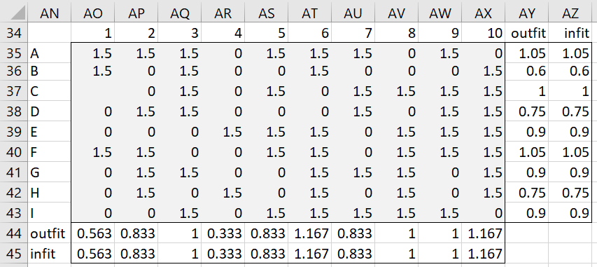
So that you can see how the calculations are done, we will pretend that the model was obtained after only one iteration and use the results from Figures 3 and 4 of Building a Polytomous Model instead of from Figure 5 of the same webpage. The results are displayed in Figure 1.

Figure 1 – Fit (after one iteration)
E.g. cell AO35 contains the formula =IF(ISNUMBER(B5),(B5-B35)^2/P35,””). The other cells in range AO35:AX43 are filled in by highlighting this range and pressing Ctrl-R and Ctrl-D.
The outfit value for the ability of subject A (cell AY35) is calculated via the formula =AVERAGE(AO35:AX35). Similarly, the outfit value for the difficulty of item 1 (cell AO44) is calculated by =AVERAGE(AO35:AO43).
The infit value for the ability of subject A (cell AZ35) is calculated via the formula =SUMSQ(AB35:AK35)/Z35. Similarly, the infit value for the difficulty of item 1 (cell AO45) is calculated by =SUMSQ(AB35:AB43)/P44. While the infit and outfit values are equal after one iteration, this won’t be true for subsequent iterations.
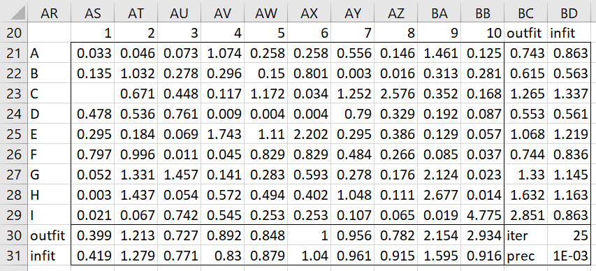
The fit output for the model after 25 iterations, i.e. the fit for the results in Figure 5 of Building a Polytomous Model, is shown in Figure 2.
Figure 2 – Fit for UCON polytomous Rasch model
Interpretation
The fit statistics measure the amount of distortion of the measurement system. The expected value of these statistics is 1.0. Values less than 1.0 typically indicate overfitting (i.e. the model too closely captures the specific data and is less likely to capture the situation in general). Values greater than 1.0 indicate unpredictability.
Some rules-of-thumb regarding the fit statistics:
- Ideally, you should prefer fit values between about .5 and 1.5 (although we will use 1.3 as the cutoff).
- Address high fit values before low fit values (eliminating high fit values will likely also eliminate low fit values). Values larger than 2 are suspect, even values between 1.5 and 2.0 can be problematical.
- Outfit values farther from 1.0 are less of a problem than Infit ones (i.e. although outfit issues are more troubling than infit issues, it is easier to eliminate outfit problems than infit problems)
- To evaluate the impact of a misfit, delete the observation, subject, or item and rerun the Rasch model. In particular, replace a misfit observation by a blank, and remove a misfit subject or item.
Examples Workbook
Click here to download the Excel workbook with the examples described on this webpage.
References
Linacre J.M. (2002) What do Infit and Outfit, Mean-square and Standardized mean? Rasch Measurement Transactions, 2002, 16:2 p.878
https://www.rasch.org/rmt/rmt162f.htm#:~:text=Polytomous%20fit%20statistics.,sensitive%20or%20information%2Dweighted%20fit.&text=Outfit%20means%20outlier%2Dsensitive%20fit,person%2C%20and%20vice%2Dversa.
Winsteps (2020) Fit diagnosis: infit outfit mean-square standardized
https://www.winsteps.com/winman/misfitdiagnosis.htm


