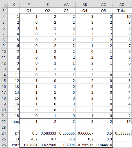
To deal with partial credit, we need to use a weighting factor. This is the argument mx in the ITEMDIFF and ITEMDISC functions described in Real Statistics Item Analysis Functions.
Example
Example 1: Find the difficulty, discrimination index (assuming a cutoff of 27%), and the point-biserial correlation coefficient for each of the five questions in a test based on the data in Figure 1 where row 22 shows the maximum credit assigned to each question. The maximum score for the whole test is the sum of these values, namely 10 (cell AD22).
Figure 1 – Item Analysis with partial credit
We will focus on Q5. The calculations for the other questions are similar.
Difficulty
The difficulty for Q5 can be calculated by either of the following formulas:
=SUM(AC4:AC21)/(COUNT(AC4:AC21)*AC22)
=ITEMDIFF(AC4:AC21,AC22).
Note too that the overall difficulty for the whole test is .583333 (cell AD24), as calculated by the formula =SUM(AD4:AD21)/(COUNT(AD4:AD21)*AD22) or =ITEMDIFF(AD4:AD21,AD22).
Discrimination Index
Since there are 18 questions and the cutoff is 27%, there are 18 ∙ .27 = 4.86 subjects in the high-skilled and low-skilled groups. We round this figure up to the nearest integer, namely 5, and so the high-skilled group consists of the subjects in rows 4 through 8, and the low-skilled group consists of the subjects in rows 17 to 21.
You can calculate the discrimination index for Q5 by using either of the following formulas:
=(SUM(AC4:AC8)-SUM(AC17:AC21))/(COUNT(AC4:AC8)*AC22)
=ITEMDISC(AC4:AC21,$AD4:$AD21,,AC22)
Note that the first of these works properly since the borders between the high, medium, and low-skilled subjects don’t overlap.
Point-biserial correlation
The correlation between the scores for Q5 and the total scores is calculated as usual by the formula
=CORREL(AC4:AC21,$AD4:$AD21)
We can also obtain the results for this example using the Item Analysis data analysis tool, as shown in Item Analysis Data Analysis Tool.
Examples Workbook
Click here to download the Excel workbook with the examples described on this webpage.
Links
↑ Test theory and item analysis
References
Matlock-Hetzel, S. (1997) Basic concepts in item and test analysis. Texas A&M
http://ericae.net/ft/tamu/Espy.htm
Office of Educational Assessment (2016) Understanding item analysis. University of Washington
http://www.washington.edu/assessment/scanning-scoring/scoring/reports/item-analysis/
Vallejo-Elias, J.(2016) Interpretation of discrimination data from multiple-choice test items
No longer available online
Albano, A. (2016) Introduction to educational and psychological measurement, Course Notes. University of Nebraska-Lincoln
https://digitalcommons.unl.edu/cgi/viewcontent.cgi?article=1005&context=prtunl

Hi Charles!
Your guides and free resources are incredible — thank you so much for sharing these.
Re: item analysis, is there a good way in Excel where you can select certain questions (ideally via manually-entered question filters) from a master list, and then have an item analysis run based on those selected questions?
For example, I have a list of questions from multiple exams, but only want to run an item analysis on questions (across all exams) that have a “cultural competence” and “ethics” tag.
This would be really useful, but I’m not sure how this might look in practice (especially being able to filter questions based on one or more tags).
Thank you!
Hello Mia,
Thank you for your kind words about Real Statistics.
The following is an outline of how to address the issue you raise in your comment.
1. The challenge here is how to organize the data to make this possible. Let me provide a simple example where you only want to use one item analysis statistic. Let’s suppose that this statistic is calculated by the formula =XYZ(R1) where R1 is a row range. Now suppose that we have a 20-question multiple-choice exam given to 25 students. Now suppose we place the answers for each of the 25 students in columns A through Y and the answers to each question in rows 1 through 20. We can also use range AB1:AB20 to contain the correct answers to the 20 questions. We can also use column Z to contain the total score for each of the 20 students. This can be done by placing the array formula =SUM(IF(A1:A20=AB1:AB20,1,0)) in cell Z1, highlighting Z1:Z20, and pressing Ctrl-D.
2. Now let’s suppose that we use a code for each question. To make things easier, suppose code 1 means use the XYZ function for that question and code 0 means don’t use the XYZ function for that question. Let’s suppose that we put these codes in column AD. We can now place the formula =IF(AD1=1,XYZ(A1:Y1),””) in cell AF1, highlight AF1:AF20, and press Ctrl-D. Column AF now contains the item analysis statistic that is calculated by XYZ for those questions with code 1 and a blank for those questions with code 0.
Charles
I don’t understand. Normally, each question is rated 1 for a correct answer and 0 for a wrong answer. Why Q2-Q5 have 2 and 3.