Basic Concepts
We can also use Kendall’s u (as described in Kendall’s u for Paired Comparisons) when the data are based on ranks, although the significance test for agreement is different.
Note that the minimum value for u is -1/(k-1) when k is even and -1/k when k is odd. We often prefer an agreement statistic that ranges between 0 and 1, with 0 indicating no agreement and 1 indicating total agreement. To accomplish this, we use a related statistic WT that has the desired property, namely
![]()
We can use a chi-square statistic to determine whether the population parameter corresponding to WT is significantly different from zero (indicating no agreement between the judges). The test is
![]()
where
![]()
![]()
![]()
Example
Example 1: Suppose that four judges (W, X, Y, Z) rank five wines (A, B, C, D, E) as shown in range A1:G5 of Figure 1. Use Kendall’s u to determine whether there is significant agreement between the judges.
We start by creating an n × n Preference Matrix (shown in A8:G14), where n = 5 is the number of wines (subjects) being ranked. Each cell in the preference matrix counts how many times the ranking for the wine with a row label is ranked better than the wine with a column label. Here, 1 is the rank of the best wine and 5 is the rank of the least favored wine. E.g. all four judges give wine A a better rank than wine B, and so we see that cell C9 contains a 4 (and cell B10 contains 4-4 = 0).
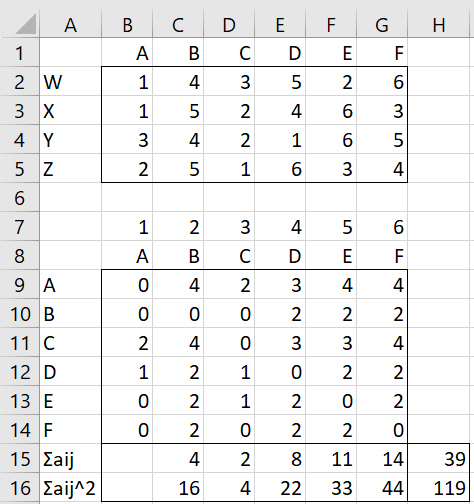
Figure 1 – Ranking data + preference matrix
We can now obtain ∑i<j aij and ∑i<j aij2 as we did for Example 1 of Kendall’s u for Paired Comparisons. Here, we show a different approach.
We obtain ∑i<j aij (in cell H15) by inserting the formula =SUM(OFFSET(C9,0,0,C7-1,1)) in cell C15, highlighting range C15:G15, press Ctrl-R, and then insert the formula =SUM(C15:G15) in cell H15.
We obtain ∑i<j aij2 (in cell H16) by inserting the formula =SUMSQ(OFFSET(C9,0,0,C7-1,1)) in cell C16, highlighting range C16:G16, press Ctrl-R, and then insert the formula =SUM(C16:G16) in cell H16.
The remaining calculations are shown in Figure 2.
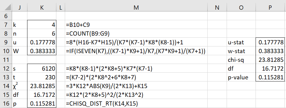
Figure 2 – Kendall’s u for paired ranks
Conclusions
Since p-value = .115281 > .05 = alpha, we cannot reject the null hypothesis (WT = 0) that there is no agreement between the judges.
We can obtain the same output by using the formula =KENDALLU(B9:G14,TRUE,FALSE), as shown in range O9:P13 (see Kendall’s u for Paired Comparisons) for a description of the KENDALLU worksheet function).
Worksheet Function
Real Statistics Function: The Real Statistics Resource Pack provides the following function for a k × n array or range R1 that contains the rankings for n subjects by k raters.
PREF_MATRIX(R1): returns an n × n preference matrix corresponding to the rankings in R1.
For Example 1, we can obtain the preference matrix shown in range B9:G14 via the formula =PREF_MATRIX(B2:G5).
Examples Workbook
Click here to download the Excel workbook with the examples described on this webpage.
Links
Reference
Siegel, S., Castellan, N. J. (1988) Nonparametric statistics for the behavioral sciences, 2nd ed.
https://psycnet.apa.org/record/1988-97307-000