LOESS Regression using Excel

LOESS (locally estimated scatterplot smoothing) regression combines aspects of weighted moving average smoothing with weighted linear or polynomial regression. LOESS is also called LOWESS, which stands for locally weighted scatterplot smoothing. We show how to perform LOESS regression in Excel.

Example

Example 1: Create LOESS regression for the data in range B2:C22 of Figure 1. This is the same data as used in the NIST example (see references below).

Figure 1 – LOESS Regression

The fitted y values for the 21 data points are shown in column E based on LOESS regression with a span of 7 points. We now show how to calculate these fitted values using the algorithm described at LOESS Regression. We also show how to create the chart on the right side of the figure.

Calculating the fitted values

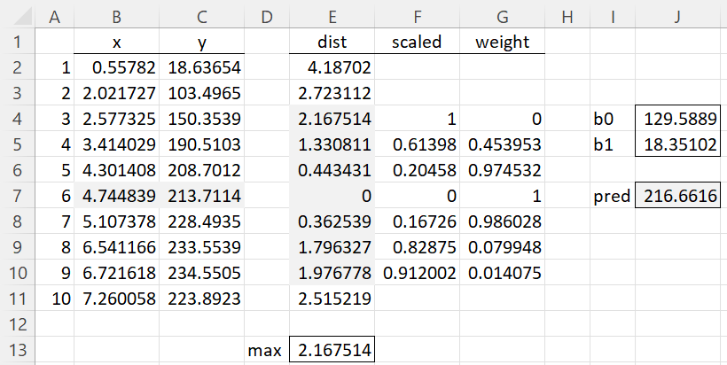
As described at LOESS Regression, for each of the 21 data points, a separate weighted linear regression is created to identify the fitted y value for that point. In Figure 2 we show how to calculate the fitted value for the 6^th data value (where x = 4.744839).

Figure 2 – Calculating the 6^th fitted value

Calculating distances

We first calculate the distance of each data point from the 6^th data point as shown in column E. E.g. the distance from the 1^st data point is 4.18702 (cell E2) using the formula =ABS(B2-B7). We see the smallest 7 distances occur in range E4:E10. With the largest being 2.167514 in cell E4. This value is calculated by =MAX(E4:E10) as shown in cell E13. Note that there is no need to display any of the distances for points 11 through 21 since their values will be larger than 2.515219, and so larger than 2.167514.

Scaled distances

We now divide each of these 7 distance values by the largest value to create the scaled distances shown in column F. E.g. cell F5 contains the formula =E5/E$13. Finally, we calculate the weights as shown in column G for each of the 7 points in the subinterval using the tricube function. E.g. cell G5 contains the formula =(1-F5^3)^3.

Weighted regression

We now perform a weighted regression using the 7 points. We can do this either using the Weighted Linear Regression data analysis tool or the WRegCoeff worksheet function (see Weighted Linear Regression). choosing the latter approach, we calculate the slope and intercept coefficients of the weighted regression by placing the array formula =WRegCoeff(B4:B10,C4:C10,G4:G10) in range J4:J5. (Note that optionally we can omit the point whose weight is zero, which will always be either the first or last point in the local subinterval, and the result will be the same).

Finally, we calculate the fitted value 216.6616 for the 6^th data point using the formula =J4+B7*J5 in cell J7. Note that this is the value that is displayed in cell E7 of Figure 1.

Calculating the fitted value for unobserved x values

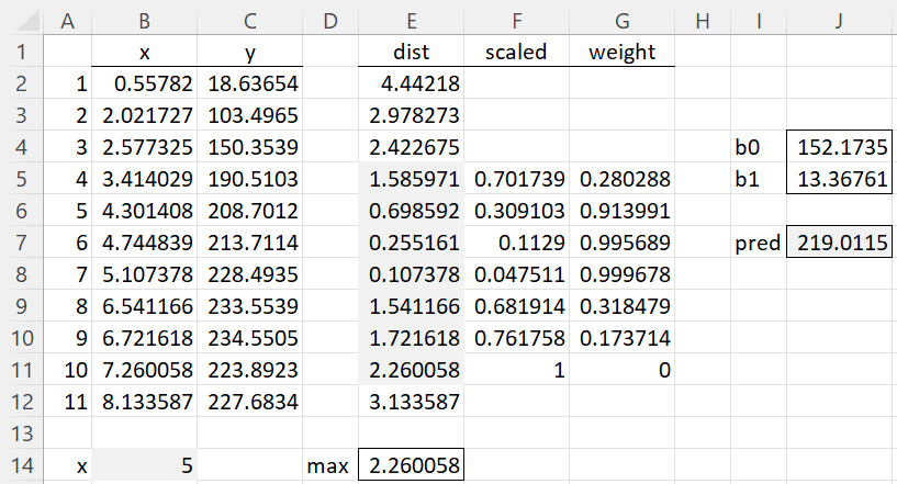
We can use the same procedure for unobserved x values. E.g. suppose that we want the fitted value at x = 5. The results are shown in Figure 3.

Figure 3 – Calculating the fitted value for new data

You need to calculate the distances from x = 5 in column E and use the closest 7 data points. We don’t need a y value for x = 5 to complete the analysis.

Worksheet Function

Real Statistics Function: The Real Statistics Resource Pack provides the following worksheet function. Here we assume that Rx is a column array or range with the x data values, Ry is a column array or range with the corresponding y values, Rx0 is a column array with any number of x values, and npts = the number of points in the span.

LOESS(Rx, Ry, Rx0, npts, deg): returns a column array with the fitted values of the LOESS regression defined by Rx, Ry, and npts for the x values in Rx0.

If Rx0 is omitted it defaults to the array values in Rx. deg = 1 (default) for weighted linear regression and deg = 2 for weighted quadratic regression. If npts is omitted (or set to zero) then npts is reset to (n+deg)/3 or the next larger integer where n = the # of elements in Rx (or Ry). Rx0 doesn’t have to be an array; it can take a scalar x value, in which case the output is the fitted y value corresponding to this x value.

The values in E2:E22 of Figure 1 can be obtained by using the array formula =LOESS(B2:B22,C2:C22,,7).

The fitted value of y = 219.0115 at x = 5 can be obtained via the formula =LOESS(B2:B22,C2:C22,5,7).

Creating the chart

We now show how to obtain the chart shown in Figure 1 assuming that we have already generated the fitted values shown in range E2:E22.

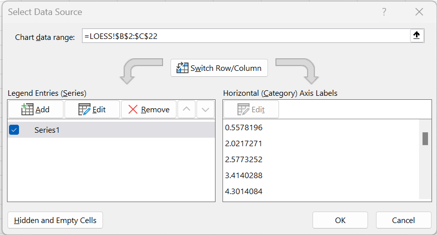
First, we create a scatter plot for the observed data in columns B and C. As usual, we highlight range B2:C22 and select Insert > Charts|Scatter. This produces the blues dots in the chart. We now need to add the red lines connecting the fitted values. To do this we click on the chart and then select Chart Design > Data|Select Data. This brings up the dialog box shown in Figure 4.

Figure 4 – Select Data Source dialog box

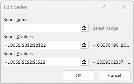
Next click on the Add button and then fill in the dialog box that appears with the fitted data (x values in B2:B22 and y values in E2:E22) as shown in Figure 5.

Figure 5 – Add fitted values via Edit Series dialog box

After clicking on the OK button, a second scatter plot with the fitted values in red will be added to the chart. You need to change the chart format from a Scatter Plot to a Scatter Plot with Straight Lines (and no markers). This is done by clicking any of the red points on the chart and selecting Insert > Charts|Scatter and selecting the Scatter with Straight Lines option.

Examples Workbook

Click here to download the Excel workbook with the examples described on this webpage.

References

NIST (2012) LOESS (aka LOWESS)
https://www.itl.nist.gov/div898/handbook/pmd/section1/pmd144.htm

Cleveland, W.S. (1979) Robust locally weighted regression and smoothing scatterplots. Journal of the American Statistical Association, Vol. 74, pp. 829-836.
https://sites.stat.washington.edu/courses/stat527/s13/readings/Cleveland_JASA_1979.pdf

NIST (2012) Example of LOESS computations
https://www.itl.nist.gov/div898/handbook/pmd/section1/dep/dep144.htm

Peltier, P. (2009) LOESS smoothing in Excel
https://peltiertech.com/loess-smoothing-in-excel/