Objective
Our objective on this webpage is to extend the simulation approach described in Single Server Queueing Simulation to the case where there is more than one server.
Example
Example 1: Model an M/M/s queueing system where λ = 5, μ = 6, and the number of servers s = 2 using simulation.
We show the results for the first 12 customers in the system in Figure 1.
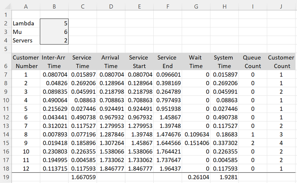
Figure 1 – Multi-server simulation
The values for row 9 of Figure 1 (customer 3) are calculated using the formulas shown in Figure 2.
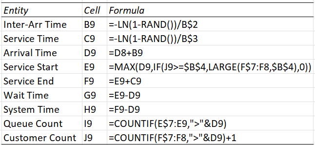
Figure 2 – Formulas from Figure 1
The formulas for the other rows are similar, except that cell D7 contains the formula =B7, and cell J7 contains the value 1. In addition, cell E7 contains the formula =D7 and cell E8 contains the formula =D8. In general, the first s entries in column E, where s = the value in cell B4, contain a similar formula.
As in Example 1 of Single Server Queueing Simulation, the system time in cell H9 can also be calculated by the formula =C9+G9, and similarly for the other values in column H. Also, the value in cell I9 can be calculated by =MAX(0,J9-B$4), and similarly for the other values in column I.
Simulation Results
From the data in Figure 1, we arrive at the values in Figure 3.
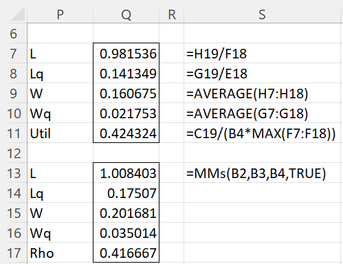
Figure 3 – L, Lq, W, Wq, ρ values
The top part of the figure is based on the simulation data. The values in the bottom part of the figure are calculated using analytic queueing theory formulas. As you can see the values are a little different.
There are several reasons for this. First, to obtain credible results from the simulation, we need to let the simulation run for a much longer period of time. 12 customers are too few. Second, the analytic formulas are based on the steady-state situation. It is unlikely that the simulation yet entered a steady state.
Note too that the simulation shown above is valid even for queueing models where the arrival and/or service rates are not exponentially distributed (i.e. G/G/s models) provided you can provide the values in columns B and C.
Worksheet Function
Real Statistics Function: The Real Statistics Resource Pack provides the following worksheet function where R1 is an array containing customer inter-arrival times, R2 is an array containing the corresponding service times and s is the number of servers.
QUEUE_SIMX(R1, R2, s, lab): returns an array with the values L, Lq, W, Wq, and Rho based on a simulation of a queueing model with s servers for m customers with inter-arrivals and service times of m customers in R1 and R2. If lab = TRUE (default FALSE) then a column of labels is appended to the output.
For Example 2, we enter the formula =-LN(RAND())/5 in cell A2 and =-LN(RAND())/6 in cell B2. We next highlight the range A2:B10001, and press Ctrl-D. Next, we enter the array formula =QUEUE_SIMX(A2:A10001,B2:B10001,2,TRUE) in range D2:E6.
The results of the simulation for 10,000 customers are shown in Figure 4. We assume that the number of iterations before a steady state is reached is small so that we can ignore these in calculating our results. The output from =MMs(5,6,2,TRUE) is shown in range D8:E12. We observe that values from the simulation are pretty close to the analytic values.
The simulation is especially useful for G/G/s models where we don’t have an analytic alternative.
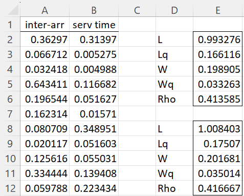
Figure 4 – Larger simulation
Examples Workbook
Click here to download the Excel workbook with the examples described on this webpage.
Reference
Leong, T-Y. (2007) Simpler spreadsheet simulation of multi-server queues. INFORMS Transactions on Education 7(2):172-177.
https://ink.library.smu.edu.sg/sis_research/215/