Basic Concepts
The M/M/1 model is a queueing process in which customers arrive at one server and wait in a queue (if necessary) until the server is available. Customers are serviced in the order in which they arrive (FIFO = first in, first out). The server services at most one customer at a time. There is no limit to the number of customers who can wait in the queue.
In the M/M/1 model, customer arrivals follow an exponential distribution at the rate of λ. Servicing also follows an exponential distribution with a service rate of μ.
The number of customers in the system = the number of customers (if any) waiting in the queue plus one if the server is occupied.
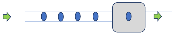
Figure 1 – M/M/1 queueing model
Balance Equations
Let pn(t) = the probability that n customers are in the system (in the queue or being served) at time t. Provided λ < μ (i.e. ρ < 1), for t sufficiently large the process enters into a steady state (aka equilibrium or balanced). Now, pn(t) doesn’t depend on t, and so we simply refer to it as pn (as described in Queueing Theory). Once in the steady state, the following equations hold
μp1 = λp0
(λ + μ)pn = λpn-1 + μpn+1
The first of these equations is based on the fact that the probability of a customer entering the system when no customers are in the system is equal to the probability that a customer exits the system when one customer is in the system.
The second (set of equations) captures the balance when one customer enters the system and another customer leaves.
Consequences of the balance equations
Note that these equations can be rewritten as
p1 = λp0/μ = ρp0
pn+1 = [(λ + μ)pn – λpn-1]/μ = (ρ + 1)pn – ρpn-1
It now follows that
p1 = ρp0
p2 = (ρ + 1)p1 – ρp0 = (ρ + 1)ρp0 – ρp0 = ρ2p0
p3 = (ρ + 1)p2 – ρp1 = (ρ + 1)ρ2p0 – ρ2p0 = ρ3p0
Continuing in this way, we see that in general
pn = ρnp0
Note too that
![]()
and so
![]()
It now follows that
p0 = 1 – ρ
Conclusions
It also follows that
pn = ρnp0 = (1 – ρ)ρn
This means that pn follows a geometric distribution with parameter 1 – ρ. Thus, the cdf is
Pn = P(l ≤ n) = 1 – ρn+1
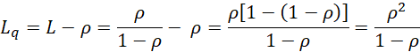
The mean number of customers in the system is
L = ρ/(1 – ρ)
and the corresponding variance is
var(l) = ρ/(1 – ρ)2
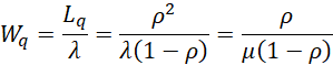
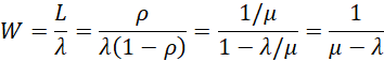
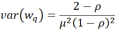
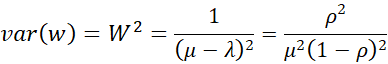
Using the properties from Queueing Theory, it follows that
The corresponding variances are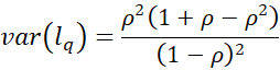
Distribution of w and wq
Once the steady state is reached, the pdf for the amount of time t that a new arrival stays in the system is given by
f(t) = (μ – λ)e–(μ – λ)t
Let w be the random variable = the amount of time a new arrival stays in the system and let wq = the amount of time a new arrival remains in the queue (waiting for service) once a steady state is reached.
For any t ≥ 0

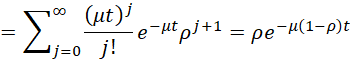
Similarly
P(w > t) = e–μ(1 –ρ)t
Thus, w is exponentially distributed with the rate parameter μ(1 – ρ).
Example
Example 1: Suppose parcels follow an M/M/1 queueing model with a mean inter-arrival time of 30 seconds (.5 minutes) and a mean service time of 24 seconds (.4 minutes). What is the average number of parcels in the system? What is the probability that there will be more than 5 parcels in the system? Also, what is the average time that a parcel waits before receiving service? What is the probability that a parcel will need to remain in the system for more than 4 minutes?
Thus, λ = 1/.5 = 2 (i.e. an average of 2 arrivals per minute) and μ = 1/.4 = 2.5 (i.e. an average of 2.5 parcels serviced per minute). We summarize the key statistics for this queueing model in Figure 1.
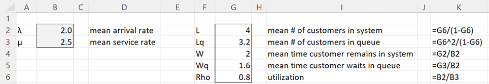
Figure 1 – M/M/1 queueing model
We see from Figure 1 that the average number of parcels in the system (once a steady state is achieved) is L = 4. The average amount of time that a parcel queues waiting for service is Wq = 1.6 minutes.
We see from Figure 2 that the probability that there will be more than 5 parcels in the system (at the same time) is 1-.737856 = 26.2144%. We can obtain the value for P5 = .737856 in cell O8 by the formula =1-G$6^(M8+1). Alternatively, it can be calculated by the formula =O7+N8. Note too that we can calculate the value for p5 in cell N8 by using the formula =(1-G$6)*G$6^M8.
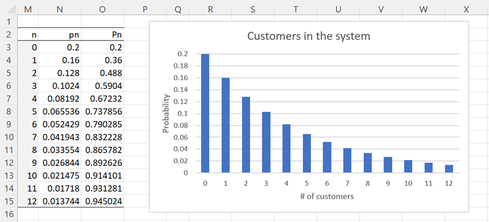
Figure 2 – Probability of n customers in the system
We see from Figure 3 that the probability that a packet remains in the system for more than 4 minutes is 13.5335% (cell R11). Note that cell R11 can be calculated by the formula =EXP(-B$3*(1-G$6)*Q11). Cell S11 can be calculated by =R11*G$6.
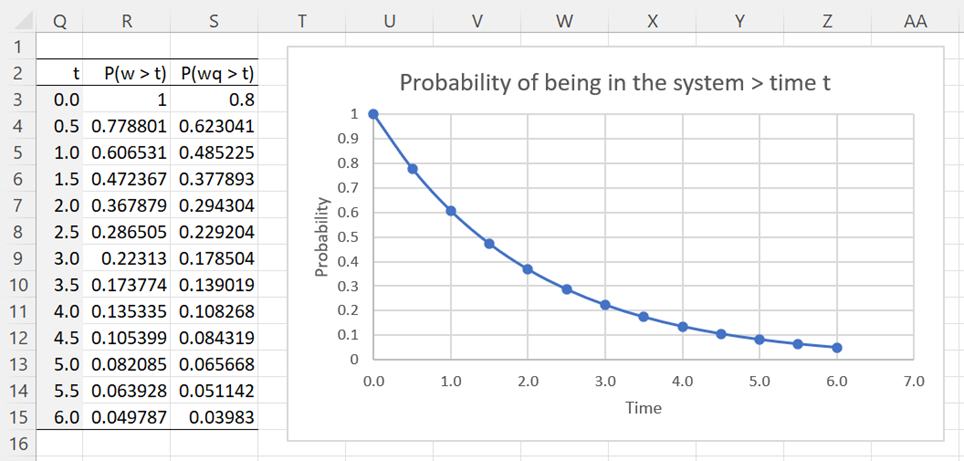
Figure 3 – Probability that wait + service time > t
Worksheet Functions
Excel Functions: The Real Statistics Resource Pack supports the following array function.
MM1X(λ, μ, lab): returns a column array with L, Lq, W, Wq, ρ for the M/M/1 queueing model with exponential arrival and service rates with a mean arrival rate of λ and mean service rate of μ.
If lab = TRUE (default FALSE) then an extra column of labels is appended to the output.
In addition, the following non-array functions are also supported.
MM1Pn(λ, μ, n, cum) = pn for the M/M/1 queueing defined by λ and μ if cum = FALSE (default) and Pn otherwise.
MM1W(λ, μ, t) = P(w > t) for the M/M/1 queueing defined by λ and μ
MM1Wq(λ, μ, t) = P(wq > t) for the M/M/1 queueing defined by λ and μ
You can obtain the values in range F2:G6 of Figure 1 via the array formula =MM1X(B2,B3,TRUE). You can obtain the values in Figure 2 by inserting =MM1Pn(B$2,B$3,M3) in cell N3 and =MM1Pn(B$2,B$3,M3,TRUE) in cell O3, highlighting N3:O15, and pressing Ctrl-D. Finally, you can obtain the values in Figure 3 by inserting =MM1W(B$2,B$3,Q3) in cell R3 and =MM1Wq(B$2,B$3,Q3) in cell S3, highlighting R3:S15, and pressing Ctrl-D.
Examples Workbook
Click here to download the Excel workbook with the examples described on this webpage.
References
Ross, S. M. (2014) Introduction to probability models, 11th Ed. Academic Press
https://ebin.pub/introduction-to-probability-models-11nbsped-0124079482-9780124079489.html
Sztrik, J. (2021) Basic queueing theory
https://irh.inf.unideb.hu/~jsztrik/education/16/SOR_Main_Angol.pdf
Shores, T. S. (2017) Queueing theory basics and models
No longer available online
Wikipedia (2023) M/M/1 queue
https://en.wikipedia.org/wiki/M/M/1_queue
un model d’application pour la file Mt/M/1
Hello Saadi,
Do you mean M/M/1?
If not, what does Mt/M/1 represent?
Charles