Basic Concepts
The M/G/1 queueing model is similar to the M/M/1 model except that the service rate follows a general distribution. This means that the service rate distribution can be any distribution with mean μ and standard deviation σ. Then assuming ρ < 1 we eventually reach a steady state, at which point the following properties hold.
Properties
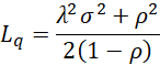
This is known as the Pollazcek-Khintichine formula. It now follows that

By Little’s Law
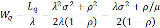
![]()
Note too that p0 = 1–ρ. Note that when servicing follows an exponential distribution, σ = 1/μ, and so the results will be equivalent to those from the M/M/1 model. Also, when servicing is deterministic, σ = 0, and so the results will be equivalent to those from the M/D/1 model.
Example
Example 1: Anna and Betty work at the supermarket packing customers’ groceries. On average Anna takes 22 seconds to do her job with a variance of 20 seconds. On average Betty takes 25 seconds to do the same type of job with a variance of 12 seconds. Assuming that customers arrive at the rate of 2 per minute following an exponential distribution, which of these two women service their customers more quickly?
The analysis is shown in Figure 1. We use minutes as the unit of measurement. Thus, cell B13 contains the value 24/60 and B14 contains 30/60. We could use seconds as the unit of measurement. In this case, we would place 24 in B13 and 30 in B14, but in that case, we would need to place 2/60 in cell B12. The results would be the same.
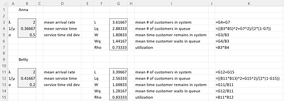
Figure 1 – M/G/1 model comparison
Despite the fact that Anna’s mean service time is lower than Betty’s, customers wait in the queue for less time when Betty is the server (Wq = 1.28167 vs. 1.44167). This is because Betty’s service time variance is less than Anna’s.
Worksheet Function
Excel Function: The Real Statistics Resource Pack supports the following array function.
MG1X(λ, μ, σ, lab): returns a column array with L, Lq, W, Wq for the M/G/1 queueing model with exponential arrivals with a mean arrival rate of λ and a service time with mean 1/μ and standard deviation of σ.
If lab = TRUE (default FALSE) then an extra column of labels is appended to the output.
You can obtain the values in range F3:G7 of Figure 1 via the array formula =MG1X(B3,1/B4,B5,TRUE).
Examples Workbook
Click here to download the Excel workbook with the examples described on this webpage.
References
Ross, S. M. (2014) Introduction to probability models, 11th Ed. Academic Press
https://ebin.pub/introduction-to-probability-models-11nbsped-0124079482-9780124079489.html
Sztrik, J. (2021) Basic queueing theory
https://irh.inf.unideb.hu/~jsztrik/education/16/SOR_Main_Angol.pdf
Shores, T. S. (2017) Queueing theory basics and models
No longer available online
Wikipedia (2023) M/G/1 queue
https://en.wikipedia.org/wiki/M/G/1_queue