We now show how to use Excel’s Solver to estimate the coefficient values that maximize the log-likelihood statistic LL (see Basic Concepts).
Example
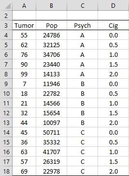
Example 1: Figure 1 summarizes the number of people who developed a tumor during the study period based on two criteria: psychological profile (A, B, or C) and the number of packs of cigarettes smoked each day (none, half a pack, one pack, one and a half packs, or two packs). For each of the 15 categories, the size of the population in that category, and the number of people who developed a tumor are listed. Develop a Poisson regression model that can be used to predict cancer in other populations.
Figure 1 – Study data
From the figure, we see, for example, that among the 24,786 non-smokers with psychological profile A, 55 developed a tumor.
Coding the Data
To create our model, we code the three psychological profiles using two dummy variables. Since the number of packs of cigarettes smoked is ordered, we retain the number of packs smoked as a numeric value. The coding is shown in Figure 2. Since our model will contain a constant term, we show these values as well (in column F).
Figure 2 – Poisson regression using Solver
Solver Set-up
Initially, we insert the value 1 for each of the coefficients in range F20:I20. The values shown in Figure 2 are those that will be obtained using Solver, as explained shortly.
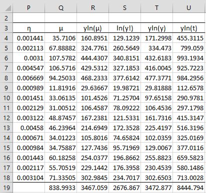
Our goal is to maximize the value of LL, labelled LLfit, (cell N14) that contains the formula =R19-Q19-S19, based on the part of the worksheet shown in Figure 3. Note that initially, LL contains the value -5925831 (based on the initial guess that all the regression coefficients are 1).
Figure 3 – Entities used to calculate LL
First, we focus on columns P through S, since these are used to calculate LL.
For example, cell P4 contains the worksheet formula =EXP(SUMPRODUCT(F4:I4,F$20:I$20)), cell Q4 contains the formula =P4*K4, cell R4 contains the formula =J4*LN(Q4) and S4 contains the formula =LN(FACT(J4)). Cells Q19, R19, and S19 contain the sums of the values in the corresponding column. As explained in Basic Concepts, LL is calculated by the formula =R19-Q19-S19 (in cell N14).
Cell T4 contains the worksheet formula =J4*LN(J4) and cell U4 contains the formula =J4*LN(B4). Cells T19 and U19 contain the sums of the values in the corresponding column. These values will be used in Poisson Regression Residuals and Goodness of Fit.
Using Solver
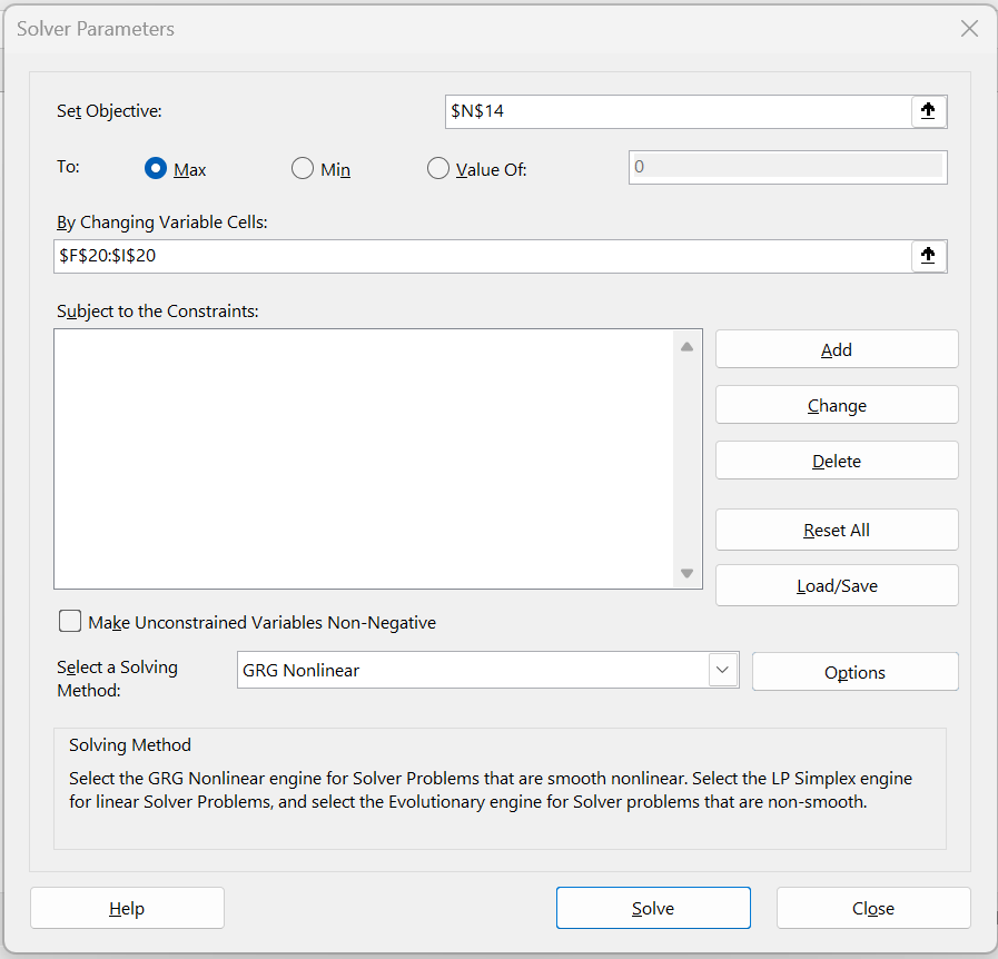
As we have done elsewhere (see Logistic Regression using Solver for example), we now use Solver to maximize LL. This is done by selecting Data > Analysis|Solver, filling in the dialog box that appears as shown in Figure 4, and pressing the OK button. The coefficients now change to the values shown in range F20:I20 of Figure 2. Also, the LL value changes to -48.8017 as shown in cell N14 of Figure 2.
Figure 4 – Solver dialog box
Standard Errors of the Coefficients
If B = [bj] is the k × 1 column vector containing the regression coefficients and μ is the n × 1 column vector of μi (scalar) values where μi = exp(xi1b1 + … + xikbk) for each i, then the covariance matrix for B is
where X is the n × k design matrix (whose rows are the Xi), and Z is the n × k matrix [zij] where zij = μi · xij. It then follows that the square root of the elements on the main diagonal of S contains the standard error of each of the regression coefficients.
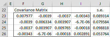
The covariance matrix for Example 1 is shown in range F23:I26 of Figure 5 using the array formula:
=MINVERSE(MMULT(TRANSPOSE(Q4:Q18*F4:I18),F4:I18))
The standard errors are shown in range J23:J26 using the Real Statistics array formula =DIAG(F23:I26).
Figure 5 – Covariance matrix
Output Summary
Thus, for Example 1, we have the coefficient table shown in Figure 6.
Figure 6 – Coefficient summary
Here, range Q23:Q26 is calculated using the array formula =TRANSPOSE(F20:I20). Cell R23 is calculated by the formula =J23, cell S23 by the formula Q23/R23, cell T23 by =2*NORM.S.DIST(-ABS(S23)), cell U23 by =Q23-R23*N$9, and cell V23 by =Q23+R23*N$9. Here cell N9 contains the formula =NORM.S.INV(1-N8/2).
From Figure 6, we see that all the coefficients are significantly different from zero.
Overdispersion
The mean and variance for a Poisson distribution are equal. In reality, the data used to create a Poisson regression model will often violate this assumption, usually with the variance being higher than the mean. To compensate for such overdispersion, a correction factor phi can be used, whereby the covariance matrix will be multiplied by phi. Phi is defined by
As can be seen in Poisson Regression Residuals and Goodness of Fit, for Example 1, φ = 1.071523. To correct for overdispersion, we need to multiply the standard error values shown in Figure 6 by the square root of φ, i.e. 1.035144. This results in the coefficient summary shown in Figure 7.
Figure 7 – Corrected coefficient summary
Examples Workbook
Click here to download the Excel workbook with the examples described on this webpage.
Links
References
Hintze, J. L. (2007) Poisson regression. NCSS
https://www.ncss.com/wp-content/themes/ncss/pdf/Procedures/NCSS/Poisson_Regression.pdf
Nussbaum, E. M., Elsadat, S., Khago, A. H. (2007) Best practices in evaluating count data, Chapter 21: Poisson regression.
http://www.academia.edu/438746
Penn State (2017) Poisson regression. STAT 504: Analysis of discrete data.
https://online.stat.psu.edu/stat504/Lesson09


