Basic Concepts
There are three partial independence models (A, BC), (B, AC) and (C, AB). We’ll look at the first of these; the others are similar. The model for (A, BC) consists of the saturated model with the λAB, λAC and λABC terms dropped. It therefore has (a – 1)(b – 1) + (a – 1)(c – 1) + (a – 1)(b – 1)(c – 1) = (a – 1)(bc – 1) degrees of freedom.
In this model A and B are independent, A and C are independent, but B and C are not independent. The probability that an observation will occur in cell ijk is
Example
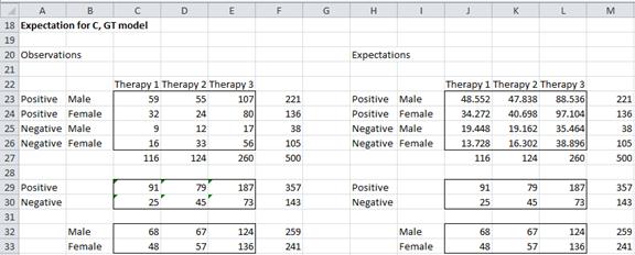
Let’s look in particular at the conditional independent model (C, GT) for Example 1 of Three-way Contingency Tables (see Figure 1).
Figure 1 – Expected frequencies for (C, GT) model
Once again, all the marginal totals for the expectations are set equal to the corresponding totals for the observations. Each of the cells in the range J23:L26 is, calculated as described above. For example, the expected frequency of a positive result for males taking therapy 1 (cell J23) is calculated via the formula =J32*M29/M27.
The degrees of freedom for this model is (2 – 1)(2∙3 – 1) = 5. From these results, we can create a table similar to that found in Figure 2 of Conditional Independence Model. From this table, we would find that χ2 (maximum likelihood) is 60.30 with 5 degrees of freedom, which is significant. This means that this model is not a good fit for the data.
Examples Workbook
Click here to download the Excel workbook with the examples described on this webpage.
Reference
Howell, D. C. (2010) Statistical methods for psychology (7th ed.). Wadsworth, Cengage Learning.
https://labs.la.utexas.edu/gilden/files/2016/05/Statistics-Text.pdf
