Bairstow’s Method

Basic Concepts

We show how to find the roots of a polynomial (with real coefficients), including complex roots, using an approach similar to Newton’s Method.

Our goal is to find all the roots of an nth degree polynomial of the form

We divide this polynomial by the quadratic

The quotient takes the form

The remainder takes the form

For any guess r and s we calculate the coefficients b_i by synthetic division, i.e. via the recursion

The objective is to find values of r and s so that h(x) = 0, i.e. b₀ = b₁ = 0.

Then, we can refine r and s as follows:

Essentially we are defining values r_i and s_i so that r_i+1 = r_i + Δr_i and s_i+1 = s_i + Δs_i. Why these c_i work in this way is shown in Theory of Bairstow’s Method using calculus (which you can skip if you like).

The goal is to keep iterating until the ratios |Δr_i/r_i| and |Δs_i/s_i| get small enough.

We use the following initial guesses

Once the values of r and s have been determined, we can determine the two roots described by x² – rx – s using the quadratic formula as follows.

We then divide the original polynomial by x² – rx – s to get a polynomial of degree n–2.

and then repeat the whole process on this polynomial. Note too that if n = 4, then the new polynomial will be of degree 2, and so we can simply use the quadratic formula to find the roots. If n = 3, the new polynomial will have the form b₃x + b₂, and so the root is x = –b₂/b₃.

Finding Roots using Solver

Example 1: Find the (real/complex) roots of the following equation using Solver.

In order to limit calculations with complex numbers, instead of finding each root individually, we find quadratic divisors as done using Bairstow’s method. The calculations are shown in Figure 1.

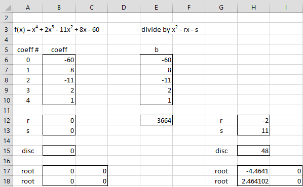
Figure 1 – Using Solver to find roots of a polynomial

Solver setup

We show the coefficients of the polynomial in range B6:B10. The parameters r and s from Bairstow’s algorithm are shown in cells B12 and B13. These are initially set to zeros. The polynomial which results from division by x² – rx – s is shown in range E8:E10 with the remainder shown in E6:E7.

Cell E10 contains the formula =B10. The formula in cell E9 is =B9+$B$12*E10. Cell E8 contains the formula =B8+$B$12*E9+$B$13*E10. The formulas in cells E6 and E7 are similar to the formula in cell E8. Our goal now is to use Solver to modify the r and s values in order to get cells E6 and E7 (the remainder after division) to become zero.

Since Solver is only able to target one cell (the Set Objective value), we place the formula =E6^2+E7^2 in cell E12 and use this as the target cell. Cells E6 and E7 only become zero when cell E12 becomes zero and vice versa.

Solver dialog box

We now select Data > Analysis|Solver and fill in the dialog box that appears as shown in Figure 2.

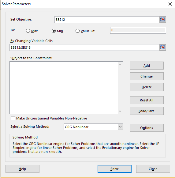
Figure 2 – Solver input

After pressing the Solve button, the spreadsheet shown in Figure 1 is modified as shown in Figure 3.

Solver output

We see that cells E6, E7, and E12 are close to zero and the values for r and s have changed to r = 0 and s = -4. This means that one of the quadratic divisors x² – rx – s of the original polynomial is x² + 4. This quadratic is zero only when ±2$latex\sqr{-1}$, which is usually written as ±2i where i = $latex\sqr{-1}$.

In general, these roots are calculated via the quadratic formula

On the spreadsheet in Figure 3, this calculation is performed in range B17:C18. First, the discriminant (i.e. the value under the square root sign in the quadratic formula) is calculated in cell B15 using the formula =B12^2+4*B13. If this value is negative, then the roots are complex numbers of the form a ± bi, with a real part a and an imaginary part b (i.e. the part that multiplies i). If the discriminant is not negative, then the roots are real numbers, each of which can be viewed as a complex number of the form a + bi where b = 0.

These values are shown in B17:C17 and B18:C18, where the value in the B cell contains the real part of the root and the value in the C cell contains the imaginary part. To accomplish this in Excel we place the formula =IF(B15>=0,(B12-SQRT(B15))/2,B12/2) in cell B17 and the formula =IF(B15>=0,0,-SQRT(-B15)/2) in cell C17. The formulas for cells B18 and C18 are identical except that we replace –SQRT by +SQRT.

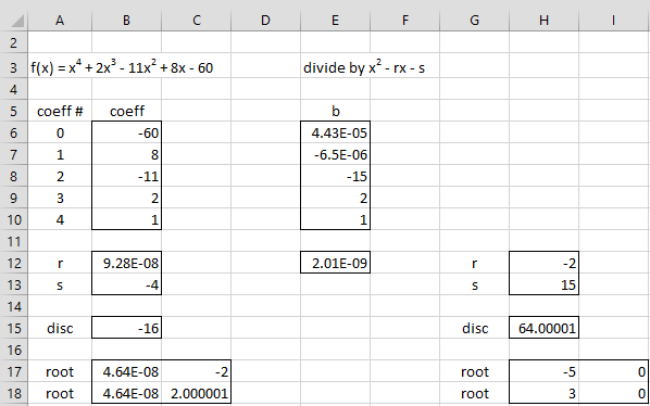
Figure 3 – Output from Solver

Conclusions

From range B17:C18, we see that the two roots are 0–2i and 0+2i (or simply ±2i). We also see from range E8:E10 that when x⁴ + 2x³ – 11x² + 8x – 60 is divided by x² + 4 the result is the polynomial x² + 2x – 15. If this were a polynomial of degree 3 or higher, then we would repeat the whole process described above based on this polynomial.

In this case, we can simply use the quadratic formula. The new r and s values are shown in cells H12 and H13. Cell H12 contains the formula =-E9, while cell H13 contains the formula =-E8. This time the resulting roots x = 3 and x = -5 are real (since the discriminant in cell H15 is positive) as shown in range H17:I18.

Thus the four roots are 3, -5, -2i, 2i.

Finding Roots using Bairstow’s Method

Example 2: Repeat Example 1 using Bairstow’s method.

The approach is similar to that used in Example 1, except that this time instead of using Solver to find the values of r and s, we use Bairstow’s method. This is shown in Figure 4.

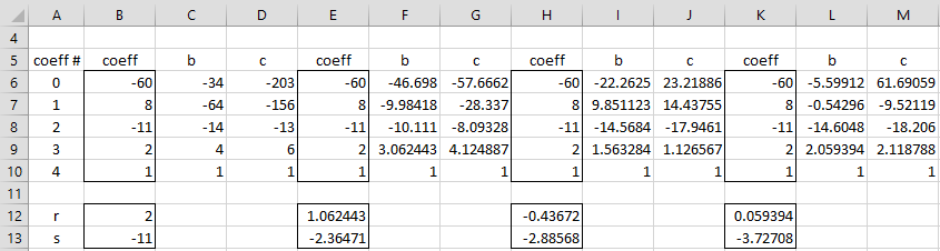
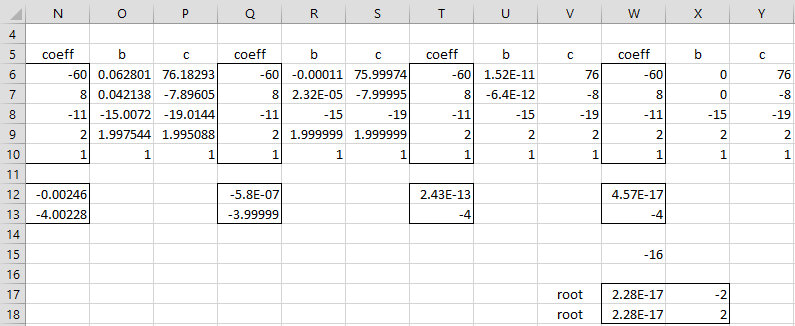
Figure 4 – Finding the roots using Bairstow’s method

Once again, we see that the process converges to roots 0 ± 2i (range W17:X18), leaving the quotient x² + 2x – 15 (range X8:X10), which yields the roots 3 and -5 using the quadratic formula, exactly as was done in Example 1 (this part is not shown in Figure 4).

Some key formulas from Figure 4 are as follows. Cells C10 and D10 contain the formula =B10, while cells C9 and D9 contain the formulas =B9+B12*C10 and =C9+B12*D10. Cells C8 and D8 contain the formulas =B8+B12*C9+B13*C10 and =C8+B12*D9+B13*D10.

Cell E12 contains the new version of r via =B12+(C6*D9-C7*D8)/(D8^2-D7*D9). Cell E13 contains the new version of s via the formula =B13+(C7*D7-C6*D8)/(D8^2-D7*D9).

The other cells contain formulas similar to these or formulas described in Example 1.

Examples Workbook

Click here to download the Excel workbook with the examples described on this webpage.

Reference

Kumar, R. (2002) Bairstow method. Numerical Analysis
https://nptel.ac.in/content/storage2/courses/122104019/numerical-analysis/Rathish-kumar/ratish-1/f3node9.html