Roots of a Polynomial | Real Statistics Using Excel

Basic Concepts

A polynomial takes the form

for some non-negative integer n (called the degree of the polynomial) and some constants a₀, …, a_n where a_n ≠ 0 (unless n = 0). The polynomial is linear if n = 1, quadratic if n = 2, etc.

A root of the polynomial is any value of x which solves the equation

Thus, 1 and -1 are the roots of the polynomial x² – 1 since 1² – 1 = 0 and (-1)² – 1 = 0.

By the Fundamental Theorem of Algebra, any n^th degree polynomial has n roots. Unfortunately, not all of these roots need to be real; some can involve “imaginary” numbers such as $\sqrt{-1}$ , which is usually abbreviated by the letter i. For example, the equation x² + 1 has the roots i and –i as can be seen by substituting either of these values for x in the equation x² + 1 = 0.

Complex Roots

The class of all numbers which includes real numbers and imaginary numbers is called complex numbers

We now give three properties of complex numbers, which will help us avoid discussing imaginary numbers in any further detail:

All complex numbers can be expressed in the form a + bi where a and b are real numbers; a is called the real part and b is called the imaginary part
If a + bi is a root of an n^th degree polynomial, then so is its conjugate a – bi
If z = a + bi then the absolute value of z is defined by |z| = $\sqrt{a^2 + b^2}$

Since a and b are real numbers, not involving $\sqrt{-1}$ , we only need to deal with real numbers.

Note that a complex number a + bi is real if b = 0. If a + bi is a real number then the definition of absolute value given above agrees with the ordinary definition since |a| = $\sqrt{a^2}$

Quadratic Polynomials

The roots of a quadratic polynomial a₂x² + a₁x + a₀ are given by the quadratic formula, namely

If the value inside the square root symbol is negative, then both roots are imaginary, while if the value inside the square root symbol is non-negative then both roots are real.

Factorization

By the Fundamental Theorem of Algebra, not only does every n^th degree polynomial have n roots, but we can use these roots as a factorization of the polynomial. More specifically, if r₁, r₂, …, r_n are these roots then we can factor the polynomial as follows

Or more succinctly

Here, we include multiple roots, i.e. roots that are repeated more than one time in the factorization. E.g. the quadratic polynomial x² + 2x + 1 = (x+1)(x+1), and so -1 is a root two times.

In the polynomial

if a₀ = 0, then it is easy to see that zero is a root, and in fact, the polynomial can be factored as

and so the n roots are zero plus the roots of the n–1 degree polynomial a_nx^n-1 + a_n-1x^n-2 +…+ a₁. In fact, if a₁ = 0, then zero is a double root and the polynomial can be factored as

If we factor out all the zero roots of the polynomial, we can assume that the constant coefficient of the polynomial that remains is non-zero.

Initial Coefficient

If all we care about are the roots of the polynomial, we can assume that the first coefficient is 1 since

has the same roots as our original polynomial and a_n/a_n = 1. Thus, where we are only concerned with roots, we can consider our original polynomial to take the form

Cubic Polynomials

In general, finding the roots of a polynomial requires the use of an iterative method (e.g. Newton’s method or Bairstow’s method, as described below). This is not necessary for linear and quadratic equations, as we have seen above. It turns out that there is a non-iterative approach for finding the roots of a cubic polynomial. See Cubic Polynomials.

Real Statistics Approach

The following Real Statistics function implements Bairstow’s Method to find all the roots of a polynomial.

Real Statistics Function: The Real Statistics Resource Pack supplies the following array function where R1 is an n+1 × 1 range containing the coefficients of the polynomial where a₀ is in the first position and a_n is in the last position.

ROOTS(R1): returns an n × 2 range where each row contains one root, and where the first column consists of the real part of the roots and the second column consists of the imaginary part of the roots

Note that the value in the last position of R1 (corresponding to a_n) does not have to be one, but it cannot be zero. The value in any other position of R1 can be zero.

Simple example

Example 1: Find the roots of

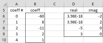
The results are shown in Figure 1

Figure 1 – Finding the roots of a polynomial

Here range D6:E9 contains the array formula =ROOTS(B6:B10).

As you can see, the four roots are 2i, -2i, -5 and 3.

Repeated roots example

Example 2: Find the roots of

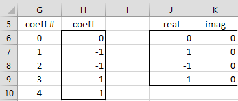
The results are shown in Figure 2

Figure 2 – Finding the roots of a polynomial

This time the roots are 0, 1, -1 (twice).

Additional arguments

The ROOTS function actually takes a number of optional parameters

ROOTS(R1, prec, iter, r, s)

prec = the precision of the result, i.e. how close to zero is acceptable. This value defaults to 0.00000001.

iter = the maximum number of iterations performed when performing Bairstow’s Method. The default is 50.

r, s = the initial seed values when using Bairstow’s Method. These default to zero.

Examples Workbook

Click here to download the Excel workbook with the examples described on this webpage.

Reference

Kumar, R. (2002) Numerical analysis
https://nptel.ac.in/content/storage2/courses/122104019/numerical-analysis/Rathish-kumar/ratish-1/f3index.html