On this webpage, we extend Newton’s root-finding approach, as described in Roots of a Continuous Function to functions with two or three variables. We begin with the Real Statistics implementation of the techniques described in Newton’s Method for use in Excel spreadsheets.
These functions take lambda function parameters. Such functions are described in Real Statistics Lambda Capabilities and Lambda Functions using Cell Formulas.
Worksheet Functions
Real Statistics Functions: The Real Statistics Resource Pack provides the following worksheet functions.
NEWTON2(R1, R2, guessx, guessy, iter, prec, incr, Rx, Ry): a 1 × 4 row array containing a root x,y of f1(x,y) and f2(x,y) along with the values of these functions at the root, based on Newton’s method using the initial guesses guessx for x and guessy for y. R1 contains the formula for f1(x,y) and R2 contains the formula for f2(x,y).
NEWTON3(R1, R2, R3, guessx, guessy, guessz, iter, prec, incr, Rx, Ry, Rz): a 1 × 6 array containing a root x, y, z of f1(x,y,z), f2(x,y,z) and f3(x,y,z) along with the values of these functions at the root, based on Newton’s method.
Rx contains the address of the cell in R1 (and R2 or R3) that corresponds to x. Ry contains the address of the cell in R1 (and R2 or R3) that corresponds to y. Rz contains the address of the cell in R1 (and R2 or R3) that corresponds to z. If Rx is omitted, then the first address in R1 is used for x. If Ry is omitted, then the second address in R1 is used for y. Similarly, if Rz is omitted, then the third address in R1 is used for z.
iter (default 100) = the maximum number of iterations. The algorithm will terminate prior to iter iterations if the error is less than some value based on prec (default .0000001).
Since this approach uses the Real Statistics function DERIV to estimate the derivative of the function f(x), the incr parameter used by DERIV needs to be specified (default .000001); See Numerical Differentiation.
Example
Example 1: Find a root for the two functions f1(x,y) = y – ex and f2(x,y) = x2 + ln y – 1.
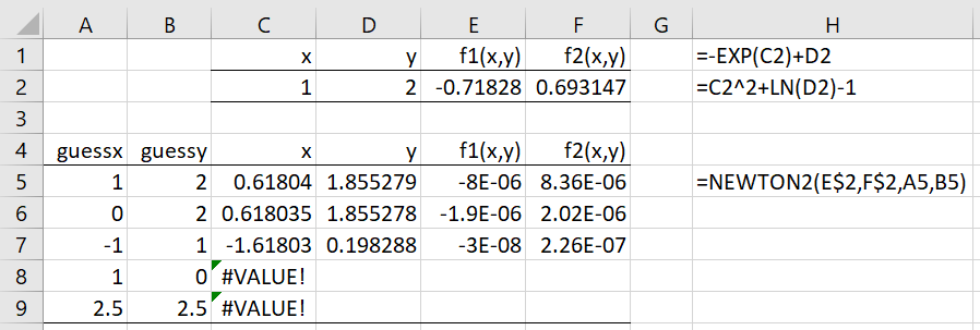
We define these functions in cells E2 and F2 of Figure 1. Here E2 contains the formula shown in H1 and F2 contains the formula shown in H2.
Figure 1 – Finding a solution to two equations in two unknowns
If we take the initial guesses x = 1 and y = 2, we get the solution x = .61804 and y = 1.855279 using the array formula shown in cell H5 in range C5:F5. We get the same solution using the initial guesses x = 0 and y = 2, as shown in row 6. If we use the initial guesses x = -1 and y = 1, we get a different solution, as shown in row 7.
If we use the initial guesses x = 1 and y = 0, we don’t get a solution, as shown in row 8. This is because ln(0) is undefined. We also see the initial guesses x = 2.5 and y = 2.5 don’t converge to a solution, even though the two functions are defined for these initial guesses. The problem here is that after one iteration the estimate for y becomes negative, which is a problem since ln(y) is also undefined for negative values of y.
Final Observation
When there are two functions f1(x,y) and f2(x,y), the formulas used for these functions must contain references to both the x and y variables and preserve the order of these references. E.g. if f1(x,y) = ey and f2(x,y) = x2 + ln y – 1, where default values for the x and y variables are used, then you need to treat the first function as f1(x,y) = 0x + ey (or something similar).
In this way, the first cell address in the formula for f1(x,y) will refer to x and not to y (since this is the order in the second function). The same applies when there are three functions.
Examples Workbook
Click here to download the Excel workbook with the examples described on this webpage.
Links
↑ Roots of a continuous function
Reference
Wikipedia (2021) Newton’s method
https://en.wikipedia.org/wiki/Newton%27s_method
