Numerical Integration Function

On this webpage, we show how to employ the various integration techniques described in Numerical Integration in Excel.

Worksheet Function

The following worksheet function takes a lambda function parameter. Such functions are described in Real Statistics Lambda Capabilities and Lambda Functions using Cell Formulas.

Real Statistics Function: The Real Statistics Resource Pack provides the following function.

INTEGRAL(R1, lower, upper, iter, ttype, Rx) = the integral ∫f(x)dx between lower and upper where R1 is a cell that contains a formula that represents the function f(x). Rx optionally contains a cell address for x (if omitted it defaults to the first cell referenced in R1). If lower is omitted then -infinity is used, while if upper is omitted then +infinity is used.

ttype is the estimation type (0 = Simpson’s rule, 1 = midpoint rule). iter = the number of subintervals (default 10,000).

If a #VALUE! error is returned it is quite possible that an overflow error has occurred. This can mean that the integral does not converge to a finite value. This can also occur when a large positive or negative value is returned, especially when the value of iter is set to a low number so that overflow hasn’t yet occurred.

Note that the formula in cell R1 can’t refer to any cells that in turn refer to cell Rx (or the first cell referenced in R1 if Rx is omitted).

Finite Integral Example

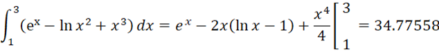
Example 1: Evaluate

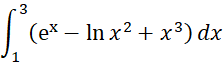
Note that

We get the same result using the formula =INTEGRAL(B5,B3,B4). The details are shown in Figure 1.

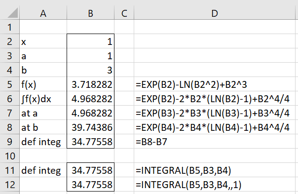
Figure 1 – Definite integral with finite bounds

Improper Integral Example

Example 2: We can evaluate the following integral

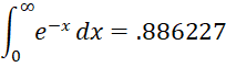
using the INTEGRAL function as shown in Figure 2.

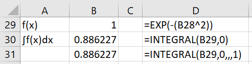
Figure 2 – Definite integral with infinite bound

Note that the formula in cell B29 cannot be replaced by =EXP(-B28^2). Due to a quirk in Excel, this would be interpreted as =EXP((-B28)^2).

Note too that if the formula in cell B29 were replaced by =EXP(B28^2), a #VALUE! error would be returned, indicating that the integral does not converge to a finite value.

Distribution Examples

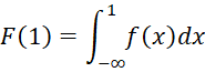
Example 3: Find the cdf at x = 1 for a normal distribution with mean 0 and standard deviation 2 by integrating the pdf.

The result is shown in Figure 3. Here, f(x) is the pdf at x and F(x) is the cdf at x.

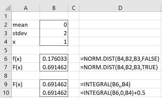
Figure 3 – Integrating to find the cdf from the pdf

Cell B6 shows that the pdf at x = 1 is .176033 and cell B7 shows that the cdf is .691462.

We can get the same value for the cdf by using the formula

as shown in cell B9. We can also get the same result using finite limits, as shown in cell B10.

Example 4: Find the value of F(2)-F(1) where F(x) is the cdf for Example 3.

We calculate this value in several ways, as shown in Figure 4.

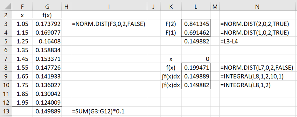
Figure 4 – Midpoint rule for integration

On the left side of the figure, we show how to manually calculate the definite integral ∫f(x)dx from x = 1 to x = 2 by using the midpoint rule with 10 subintervals to obtain the value .149889. Here, delta = (2-1)/10 = .1.

Using the INTEGRAL function, we obtain the same value as shown in cell L9. We can obtain a more accurate value of .149882 by using more subintervals. We can also obtain this value directly using the NORM.DIST function, as shown in range L3:L5.

Integral without an analytic solution

Example 5: Evaluate

for x = 4, 5, and .5.

This integral doesn’t have an analytic solution, but it turns out to be the gamma function Γ(x). We show how to use the INTEGRAL function to evaluate this integral at the three specified values in Figure 5.

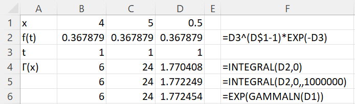
Figure 5 – Evaluation of the gamma function

This is done by placing the formula B3^(B$1-1)*EXP(-B3) in cell B2, highlighting the range B2:D2, and pressing Ctrl-R. Note that the function f(t) in row 2 is a function of t and not of x. This is accomplished by using a $ in the address (e.g. D$1 for the case where x = .5).

The integral calculates Γ(4) = 3! = 6 and Γ(5) = 4! = 24, as expected. Γ(.5) = √π = 1.7722452, but the value produced by the INTEGRAL function with the default number of iterations (cell D4) is only correct to two decimal places. If the number of iterations is increased to one million, then the accuracy increases to 3 decimal places.

Examples Workbook

Click here to download the Excel workbook with the examples described on this webpage.

References

Wikipedia (2021) Numerical integration
https://en.wikipedia.org/wiki/Numerical_integration

Scherfgen, D. (2021) Integral calculator
https://www.integral-calculator.com/#

Stubner, R. (2019) Numerical integration over an infinite interval in Rcpp (part 2). R-bloggers.
https://www.r-bloggers.com/2019/07/numerical-integration-over-an-infinite-interval-in-rcpp-part-2/