Kruskal Algorithm
We show how to construct a minimum spanning tree (MST) for a connected graph using the Kruskal algorithm.
Step 0: We begin by sorting all the edges in the graph by weight from lowest to highest. Next, we construct the MST in m steps where m = the number of edges in the graph. We start with a forest of n trees, where each tree consists solely of one of the n nodes in the graph.
Step 1: We evaluate the first edge in the graph (i.e. the edge with the lowest weight). Here, we determine whether to combine the tree containing one node on this edge with the tree containing the other node on this edge. If so, this edge becomes part of the MST. More specifically, we link these two trees via the edge under consideration provided the result is still a tree (i.e. no cycle is formed).
Step 2: We then proceed to the second edge and repeat the process described in step 1.
Steps 3 to m: We continue in this way until we have evaluated all m edges, at which point we obtain an MST.
Algorithm Details
In order to carry out these steps in an efficient way, we use two functions: p (parent) and r (rank). p is used to create a linked list of nodes that form one of the trees in the forest. p(i) = the parent node of node i, but when p(i) = i, this means that node i has no parent and so is the root of the tree. We initially set p(i) = i for all the nodes, which indicates that we start with a forest of one-node trees.
Determining the root
At any step in the process, we can determine the root of the tree that contains node i by first finding p(i). If p(i) = i then i is the root. If not, we look at the parent of p(i), i.e. p(p(i)). If p(p(i)) = p(i) then p(i) is the root of the tree that contains i. If not, then we look at p(p(p(i))) to determine whether p(p(i)) is the root of the tree containing i. We continue in this fashion until the root is found.
Actually, when we have found the root k of the tree that contains i, to save time in the future, we collapse the linked list so that all the nodes in the tree from i to k point to k and not to its direct parent. E.g. if k is p(p(p(p(i)))), then we set p(i) = k, p(p(i)) = k and p(p(p(i))) = k.
At each step in the algorithm, we find the root of each of the two nodes on the edge under consideration (as described above). If these nodes have the same root, then we don’t combine the trees (otherwise a cycle would result). In this case, this edge does not become part of the MST.
If instead, the roots are not the same, then this edge does become part of the MST and we do link the two trees. To accomplish this, we use the rank function.
r(i) = the rank of node i. When we combine trees we need to determine which tree supplies the root of the combined tree. This is done by using the root with the higher rank. We initially set r(i) = 0 for all nodes.
Suppose that the edge under consideration is (h, k) and suppose that the root of h is i and the root of k is j. Then if r(i) > r(j), we set p(j) = i, while if r(j) > r(i), then we set p(i) = j. If r(i) = r(j), then we set p(i) = j and we set r(j) = r(j) + 1.
Example
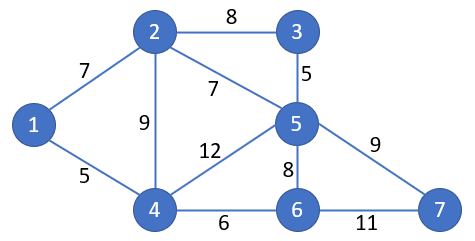
Example 1: Find the minimum spanning tree for the graph described in Figure 1.
Figure 1 – Network Diagram for Example 1
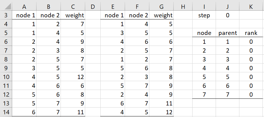
The Excel representation of this graph is shown on the left side of Figure 2. This range is sorted by weights to obtain the representation shown in the middle of the figure using the array formula =QSORTRows(A4:C14,3). The right side of the figure shows the initial values for the p() and r() functions.
Figure 2 – Initialization
First 8 steps
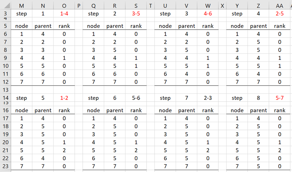
Figure 3 shows the first 8 steps of the algorithm. We have highlighted the edges that become part of the minimum spanning tree in red. The remaining 3 steps in the algorithm don’t add any further edges to the minimum spanning tree.
Figure 3 – Next 8 steps
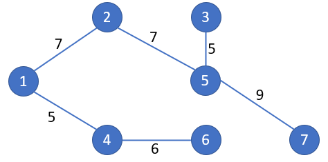
The resulting minimum spanning tree is shown in Figures 4 and 5.
Figure 4 – Network Diagram for MST
Figure 5 – MST in Excel format
Note that the number of edges in the minimum spanning tree is always one less than the number of nodes.
Worksheet Functions
Real Statistics Function: The Real Statistics Resource Pack contains the following array function where R1 is an array with three columns where the first two columns contain the node numbers of the graph in ascending order and the third column contains the weights for the edge defined in each row.
MSTKruskal(R1, brief): returns an array with the rows from R1 that constitute an MST for R1 using the Kruskal algorithm assuming that brief = FALSE (default).
When brief = TRUE, then a column array is output with the same number of rows as R1. For each row in R1, the corresponding row in the output contains a 1 if that row (in R1) is in the MST. It contains a 0 if that row is not in the MST.
For the graph defined on the left side of Figure 2, we can use the array formula =MSTKruskal(A4:C14) to obtain the MST shown in Figure 5.
Examples Workbook
Click here to download the Excel workbook with the examples described on this webpage.
Links
References
Cormen, T. H., Leiserson, C. E., Rivest, R. L. (1992) Introduction to algorithms. MIT Press.
https://mitpress.mit.edu/books/introduction-algorithms-third-edition
Barnwal, A. (2020) Kruskal’s minimum spanning tree algorithm, Greedy Algo-2. GeeksforGeeks
https://www.geeksforgeeks.org/kruskals-minimum-spanning-tree-algorithm-greedy-algo-2/
Wilson, R. J. (1996) Introduction to graph theory. 4th ed. Prentice Hall
https://webhomes.maths.ed.ac.uk/~v1ranick/papers/wilsongraph.pdf
Good morning Professor,
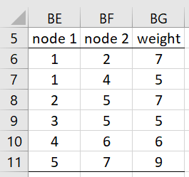
building MST of figure 3, how can I calculate the rank? Why, in step 5, does the rank of “5” increase to “2”? Why isn’t the rank of “4” increasing to “2”?
All in all, the “1-4-6” tree is similar to the “2-5-3” tree.
Best regards, Roberto
Hello Roberto,
For step 5, look at the results from step 4. We process the link with initial node 1 and terminating node 2. We observe that the parent of node 1 is 4 and the parent of node 2 is 5. Since nodes 4 and 5 have the same rank, namely 1, as described in the paragraph before the Examples heading, we change the parent of the initial node to the parent of the terminating node, i.e. 5, and increment the rank of the parent of the terminating node, i.e. the rank of node 5 changes from 1 to 2. We don’t change the rank of node 4.
Charles