On this webpage we demonstrate how to use the Real Statistics worksheet functions MGRADIENT and MGRADIENTX to identify the value of X that minimizes the function f(X). See Gradient Descent for more information about these two functions and the gradient descent algorithm.
Simple Example
Example 1: Find the values of x and y that minimize the following function:
f(x, y) = x – y + 2xy + 3x2 + y2
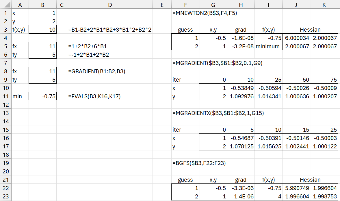
We show the results in Figure 1 using the Newton-Raphson, BGFS and Gradient Descent approaches.
Figure 1 – Simple minimization example
First we represent f(x, y) in cell B3. Picking initial guesses of (1, 2) and using Newton-Raphson yields the solution (-.5, 1) with f(-.5, 1) = – .75 as shown on the upper right-hand side of the figure. Convergence is obtained in 3 iterations. Using BGFS we achieve convergence in 4 iterations, as shown on the bottom right-hand side of the figure.
If we use gradient descent with the fixed default learning rate of .1, using MGRADIENT, and an initial guess of (1, 2), it takes more than 25 iterations to achieve the desired output with two decimal place accuracy, and more than 50 iterations to achieve three decimal place accuracy.
If we use gradient descent with variable learning rates, using MGRADIENTX, and an initial guess of (1, 2), we obtain similar levels of accuracy with fewer iterations.
Constrained Example
Example 2: Find the values of x and y that minimize the following function:
f(x, y) = –ln (1 – x – y) – ln(x) – ln(y)
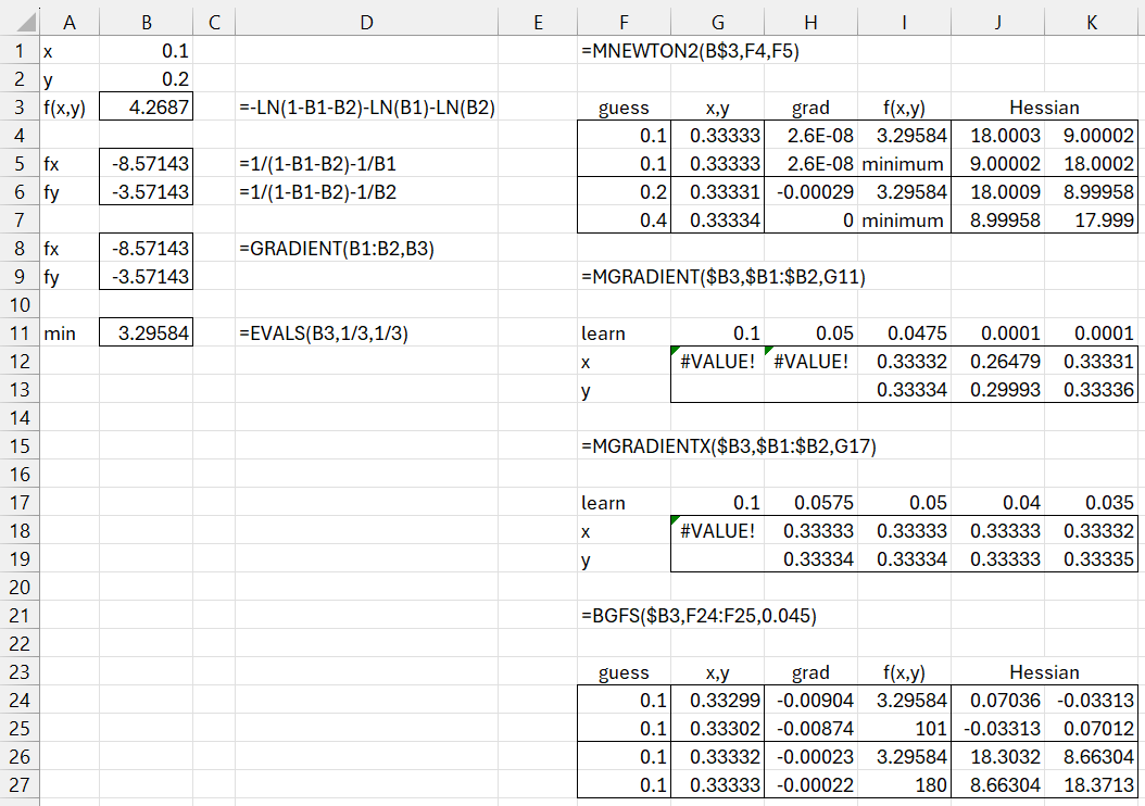
We now show the results in Figure 2 using the Newton-Raphson, BGFS and Gradient Descent approaches.
Figure 2 – Constrained minimization example
First we represent f(x, y) in cell B3. Since ln(z) is undefined for non-positive values, we observe that x and y must take positive values and x + y < 1. Picking initial guesses of (.1, .1) or (.2, .4) and using the Newton-Raphson method yields the solution (1/3, 1/3) with f(1/3, 1/3) = 3.295837 as shown on the upper right-hand side of the figure. Convergence for an initial guess of (.1, .1) is achieved in 6 iterations, while converge is achieved in 4 iterations for an initial guess of (.2, .4).
If we use gradient descent with a fixed learning rate of .1 or .05 and an initial guess of (.1, .2), we get an error value, as shown in cells G12 and H12. If we lower the learning rate to .0475, the gradient descent algorithm converges to the (1/3, 1/3) solution within the 500 default iterations. However, if we lower the learning rate to .0001, convergence is not achieved, as shown in J12:J13 after 500 iterations. If we now increase the number of iterations to 10,000, we do get convergence, as shown in K12:K13 using the array formula =MGRADIENT($B3,$B1:$B2,K11,10000).
Caution
The gradient descent algorithm with backtracking line search doesn’t converge to a solution when the initial learning rate is set to the default value of 1, or even .1, as shown in cell G18 using the formula =MGRADIENTX(B3,B1:B2,,5000). The reason for this is as follows.
In the first iteration, X0 is initialized to the values shown in B1:B2, resulting in the gradient ∇f(X0) being set to the values shown in B5:B6, and so
since α0 is initially set to 1. But as we observed earlier, f(X0 – α0∇f(X0)) is now undefined since 8.67143 + 3.77143 > 1. If instead, we initially set α0 = .0575 (or less), then
and since .592857 + .405357 < 1 we avoid this problem, and so once again obtain the (1/3, 1/3) solution.
We will fix this issue in the next release by allowing the user to set the initial value of learn to a value less than or equal to .0575. E.g., by using the formula =MGRADIENTX(B3,B1:B2,0.0575,5000). This is not possible in the current release, Rel 9.2, but will be possible in the next release, available shortly.
Finally, we see that the BGFS approach converges to a solution, using an initial learning rate of .045, accurate to 3 decimal places within the default number of 100 iterations, but the Hessian is way off. BGFS requires 180 iterations to converge to a solution for (x, y) and the Hessian near the accuracy of the Newton-Raphson method. If the initial learning rate is set to 1, as in the current release of the Real Statistics software, then no solution is found (the problem is the same as that described above for MGRADIENTX). This problem will be resolved in Rel 2.2.1 where the initial learning rate can be set by the user.
Minimizing the Rosenbrock function
Example 3: Find the values of x and y that minimize the following function:
f(x, y) = (2 – x)2 + 100(y – x2)2
This is an example of the Rosenbrock function which takes the form
f(x, y) = (a – x)2 + b(y – x2)2
for constants a and b. This class of functions is often used to test the performance of procedures that seek to minimize a multivariate function. In general, the minimum occurs at (a, a2), which for Example 3 is (2, 4).
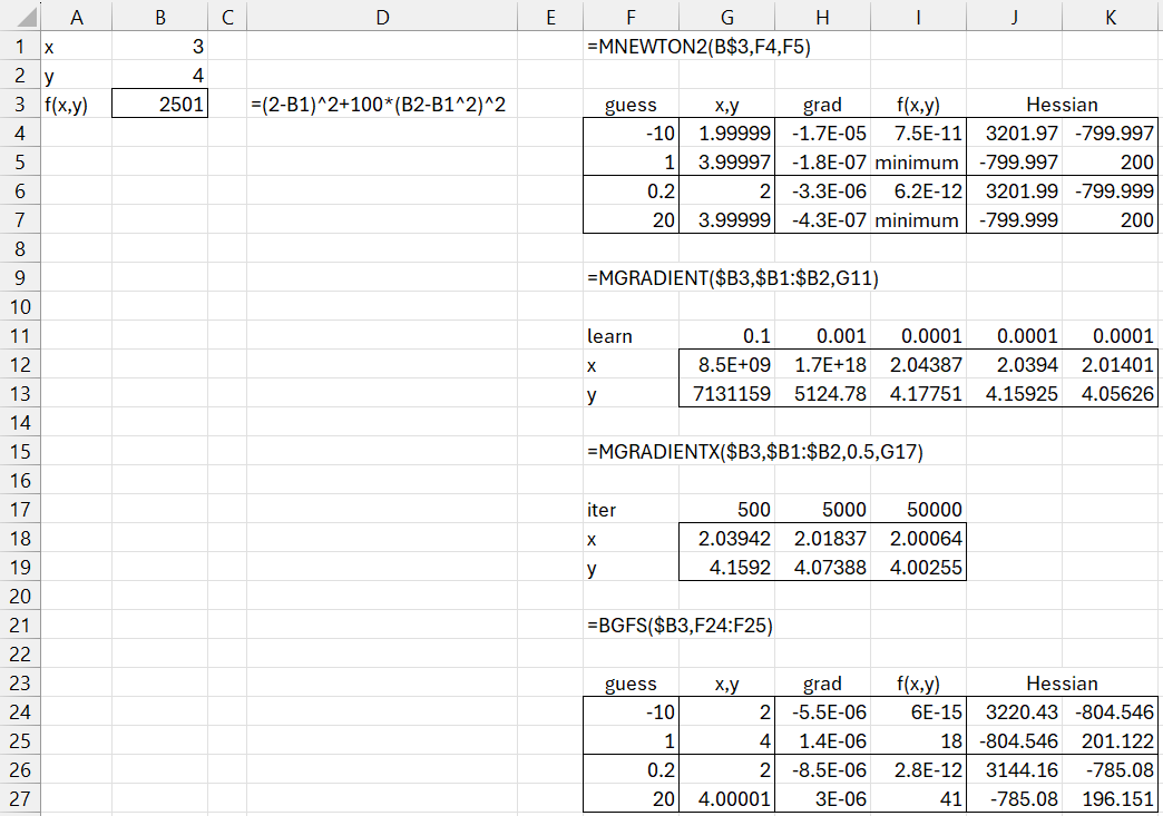
We show the results in Figure 3 using the Newton-Raphson, BGFS, and Gradient Descent approaches.
Figure 3 – Minimization of a Rosenbrock function
The solution (2, 4) is found using the Newton-Raphson method in 24 iterations when the initial guess is (-10, 1), but only 9 iterations when the initial guess is (.2, 20). Interestingly, the BGFS method converges to the solution in only 18 steps when the initial guess is (-10, 1) and 41 iterations when the initial guess is (.2, 20).
When using gradient descent with a fixed learning rate, the algorithm diverges when learn = .1 or even .001. When learn = .0001, the accuracy of the solution increases progressively as the number of iterations increases from 500 to 10,000 to 100,000 in I12:I13, J12:J13, and K12:K13. Even at 100,000 iterations the solution is only fairly accurate.
Convergence occurs more rapidly when using gradient descent with backtracking line search, as shown in rows 17. 18, and 19 of Figure 3.
Examples Workbook
Click here to download the Excel workbook with the examples described on this webpage.
Note that the workbook may be slow to open since the various spreadsheets need to perform quite a few iterations.
Links
References
Khan Academy (2024) Gradient descent
https://www.khanacademy.org/math/multivariable-calculus/applications-of-multivariable-derivatives/optimizing-multivariable-functions/a/what-is-gradient-descent
Wikipedia (2024) Gradient descent
https://en.wikipedia.org/wiki/Gradient_descent
Cao, L., Sui, Z., Zhang, J., Yan, Y., Gu, Y. (2021) Line search methods
https://optimization.cbe.cornell.edu/index.php?title=Line_search_methods
Kochenderfer, M, J., Wheeler, T. A. (2019) Algorithms for optimization
https://algorithmsbook.com/optimization/files/optimization.pdf
Wikipedia (2024) Rosenbrock function
https://en.wikipedia.org/wiki/Rosenbrock_function


