Complex Linear Equations

Basic Concepts

Suppose we have a set of n linear equations in n unknowns. As we have seen in Systems of Linear Equations, we can represent this in matrix form as

AX = C

Now suppose that A and C can have complex entries, and so the solution vector X can also have complex entries. Furthermore, we can represent any complex number z as

z = z_r + z_ci

Similarly, any complex matrix Z can be represented as

Z = Z_r + Z_ci

We now consider the following set of 2n real-valued linear equations in 2n unknowns

where

Then X-tilde is a solution to the real-valued linear equations is equivalent to X = X_r + X_ci is a solution to the original system of linear equations AX = C.

Example with a unique solution

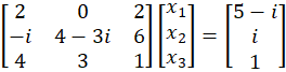
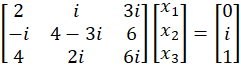
Example 1: Solve the following linear equations.

The augmented matrix in Excel format is shown in range B3:E5 of Figure 1. The same matrix in Real Statistics format is shown in range G3:N5, using the formula =ZMap(B3:E5).

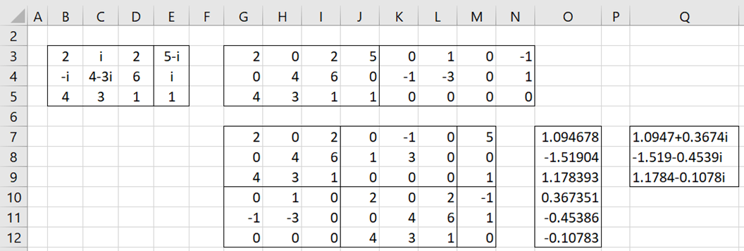
Figure 1 – Unique Solution to Complex Linear Equations

We next reformat this augmented matrix to the format required by Property 1, as shown in range G7:M12. The resulting solution to the real linear equations in G7:M12 is shown in range O7:O12 using the formula =LinEqSolve(G7:M12). We can then represent this solution vector in Excel format as shown in range Q7:Q9 with the entries rounded off to 4 decimal places. This is accomplished using the worksheet formula =ZMROUND(ZText(ZSet(O7:O9,O10:O12)),4).

Examples with non-unique solutions

Example 2: Solve AX = C with A = the matrix in range B3:D4 and C = the vector in range E3:E4 of Figure 2.

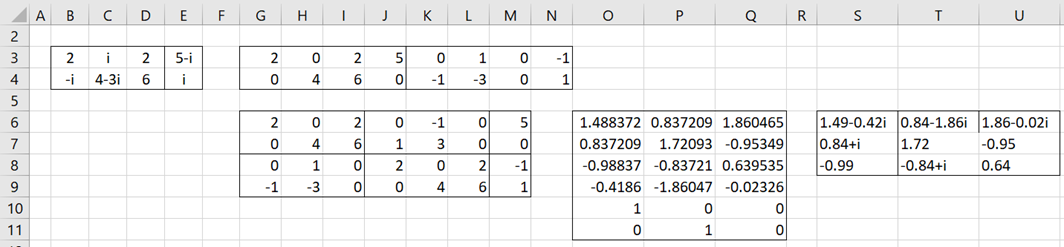
Figure 2 – Infinite number of solutions

The approach is similar to that used for Example 1. There are an infinite number of solutions all of the form

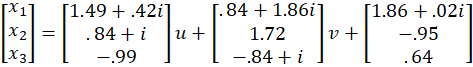
where u and v are any (complex) constants.

Example 3: Solve the following system of linear equations

Using the same approach, you will obtain the value #N/A from the resulting formula of form =LinEqSolve(R1). This means that there is no solution. This is evident since the third row of the A matrix is double that of the first row, while the entry in the third row of the C vector is not double that of the entry in the first row.

Worksheet Functions

Real Statistics Functions: The Real Statistics Resource Pack provides the following array function which automates the above process. Both the augmented matrix in R1 and the output use the Real Statistics format for complex numbers.

ZLinEqSolve(R1, prec): an array function that outputs the solution vectors for the system of linear equations defined by the augmented matrix found in the array R1. The number of rows in the output is one less than the number of columns in R1.

During Gaussian elimination, values less than prec (default .0001) are treated as zero.

If the system of linear equations does not have a solution, then the error value #N/A is returned. If there is a unique solution (including the trivial solution for a system of homogeneous equations), then the output will consist of a column array with this solution.

For Example 2, the formula =ZLinEqSolve(G3:N4) produces the output shown in Figure 3.

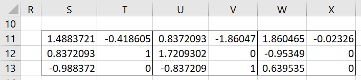
Figure 3 – Output from ZLinEqSolve

The Real Statistics Resource Pack also provides the following array function which is identical to ZLinEqSolve, except that now both the augmented matrix in R1 and the output use the Excel format for complex numbers.

IMLinEqSolve(R1, ndigits, prec): an array function that outputs the solution matrix for the system of linear equations defined by the augmented matrix found in the array R1.

If ndigits ≥ 0 (default 4), then the output vectors use numbers rounded off to ndigits decimal places. If ndigits < 0 then no rounding is used.

E.g. for Example 1, the array formula =IMLinEqSolve(B3:E5) produces the results shown in range Q7:Q9 of Figure 1. For Example 2, the array formula =IMLinEqSolve(B3:E4,2) produces the output shown in range S6:U9 of Figure 2.

Examples Workbook

Click here to download the Excel workbook with the examples described on this webpage.

References

Militaru, R. and Popa, I. (2012) On the numerical solving of complex linear systems. International Journal of Pure and Applied Mathematics. Vol 76 No. 1, pp 113-122
https://ijpam.eu/contents/2012-76-1/11/11.pdf

Brenner, S. C., Kaup, D. J. (1999) Introduction to complex numbers
https://control.dii.unisi.it/sistdin-SI/complex.pdf