Return Period and Return Level

Basic Concepts

The return period (aka recurrence interval or repeat interval), is the estimated (or tolerated) average time between extreme events such as floods, earthquakes, or landslides. If we observe or theorize that in a certain location an earthquake of say 7.0 on the Richter scale occurs on average every 100 years, then we say this is a 100-year event, usually stated as a once-in-a-century event. In any year, the probability that there will be an earthquake of this severity is then 1/100 = 1%.

As usual, this doesn’t mean that an earthquake of this severity will occur exactly once every 100 years. 1% is the expected occurrence. An earthquake of this severity may not occur even once in the next 100 years, or it may occur twice in the next 100 years. As we know the probability that it will occur at least once in 100 years is 1 – (99/100)¹⁰⁰ = 63.4%. The probability that it will occur exactly once in 100 years is C(100,1)(.01)¹(.99)⁹⁹ = 37.0%.

Here, we are assuming that the probability of an extreme event in any year is the same as the probability of such an event in any other year. This is equivalent to saying that the time series of events being measured is stationary. If, say, the event under consideration is the maximum water level at a levy, then stationary means that we cannot detect a trend in the water level from year to year. Clearly, climate change may undermine such an assumption.

Resiliency

To gauge the resiliency to an extreme event over a period of r years, we check to see whether the F(x) > 1 – 1/r where x is the putative maximum value of some variable (e.g. the height of water at a levy or the size of earthquakes on the Richter scale) in a given time period (say in a year) and F(x) is the cumulative distribution function (cdf) at x. It turns out that the Generalized Extreme Value (GEV) distribution is the appropriate distribution in many cases.

Similarly, to determine what is an acceptable value of x to endure extreme events over the course of r years, called the return level, we use the inverse function F^-1(1–1/r). We illustrate these concepts via Example 1.

Example

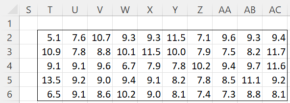
Example 1: Figure 1 contains the maximum annual water level at a certain dam over the past 50 years. The current height of the dam is 13.5, which means that the dam held over the past 50 years, although in one year it barely held. Do we expect that the dam will hold for the next 100 years? How high does the dam need to be to hold for the next 100 years?

Figure 1 – Historical water levels over 50 years

The data in Figure 1 is identical to that shown in Figure 1 of Fitting a GEV Distribution using MLE, and so we will assume that this situation can be modeled by a GEV distribution with the MLE parameters shown in range K2:K4 of Figure 3 of Fitting a GEV Distribution using MLE (using the GEV_FIT function), namely mu = 8.464309, sigma = 1.467846, xi = -0.20077.

The probability that the dam won’t hold in any year over the course of 100 years is therefore

1-GEV_DIST(13.5, 8.464309, 1.467846, -.20077, TRUE) = 0.2982%

Also, the required height is

GEV_INV(.99, 8.464309, 1.467846, -.20077) = 12.87217

This means that the dam is already high enough to achieve this objective.

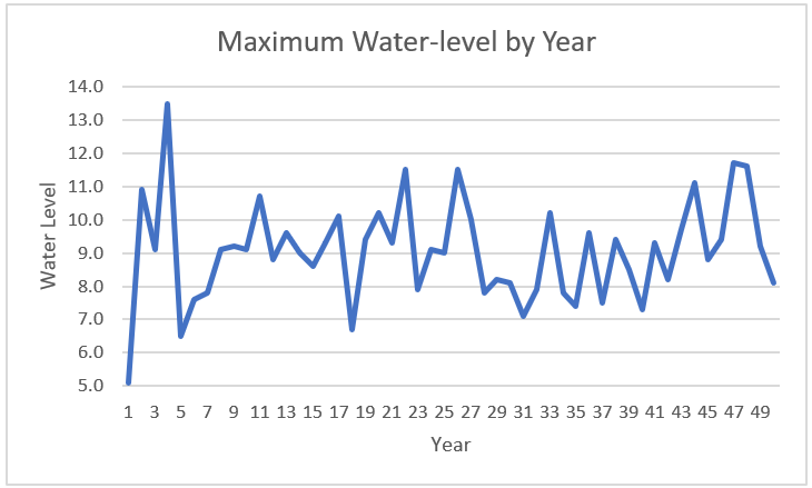
Finally, note that the graph of the historical data displayed in Figure 2 shows a random pattern with no trend or seasonality.

Figure 2 – Water level by Year

Examples Workbook

Click here to download the Excel workbook with the examples described on this webpage.

References

Wikipedia (2021) Return period
https://en.wikipedia.org/wiki/Return_period

Fawcett, L. (2012) Classical model for extremes
http://www.mas.ncl.ac.uk/~nlf8/teaching/mas8391/background/chapter2.pdf