Real Statistics Ordinal Regression Support

The Real Statistics Resource Pack provides support for the proportional odds model of ordinal regression using Newton’s method, as described in Proportional Odds Model.

Worksheet Functions

Real Statistics Functions: The Real Statistics Resource Pack provides the following array function where R1 contains data in either raw or summary form.

OLogitCoeff(R1, r, lab, head, alpha, iter, guess) – calculates the ordinal regression coefficients using Newton’s method for the data in R1. For each coefficient, the output also includes the standard error, Wald statistic, p-value, and 1 – α confidence interval. If head = TRUE then R1 includes column headings.

For each row in R1, the initial n columns specify values for the independent variables. If r = 0, then R1 is in raw data format with n+1 columns where the last column of R1 contains category numbers (integer values starting with 1); otherwise, R1 is in summary format and contains n+r columns where the last r columns specify the counts for each category 1, 2, …, r.

The output specifies the coefficients. If there are r categories, then the first r-1 entries specify the coefficients a₁, …, a_r-1, and the remaining n entries specify the coefficients b₁, …, b_n. If guess is included then the coefficients in the n+r-1 × 1 column array guess are used as the initial values in Newton’s method; if this argument is omitted then the function decides internally what initial values to use.

alpha specifies the significance level (default .05) and iter (default 20) specifies the number of iterations used by Newton’s method.

Related worksheet functions

The Real Statistics Resource Pack also provides the following array functions where R1 contains data in either raw or summary form and Rc is a column array that contains the ordinal regression coefficients, where R1, Rc, and r are as described above. We will assume that there are n independent variables and r categories 1, 2, …, r (and so Rc has n+r-1 rows).

OLogitCov(R1, Rc, r) – returns the covariance matrix corresponding to the regression coefficients in Rc based on the data in R1. 

OLogitConverge(R1, Rc, r) – returns the F column array described in Property 2 of Proportional Odds Model. The values in this array should all be close to zero if Rc provides a sufficiently accurate representation of the ordinal regression coefficients. Note that if B adequately represents the true regression coefficients and C represents the covariance matrix for these coefficients (e.g. as calculated by OLogitCov) then per Property 2 of Proportional Odds Model, B – CF should be very close to zero.

OLogitLL(R1, Rc, r, lab) – returns a column array with the values LL, LL0, chi-square test results (chi-square stat, df, and p-value), R-square (McFadden, Cox and Snell, Nagelkerke versions), AIC and BIC. If lab = TRUE (default FALSE) then an extra column is appended to the output which contains labels.

The Real Statistics Resource Pack provides the following non-array function:

OLogitCorrect(R1, Rc, r) = the fraction of the observations in R1 for which the ordinal regression model based on the coefficients in Rc correctly predicts the observed outcome (i.e. where the observed category is the one with the highest probability per the model)

The Real Statistics Resource Pack also provides the following array functions:

OLogitSummary(R1, head) – array function that takes the raw data in R1 and outputs an equivalent array in summary form. If head = TRUE then R1 includes column headings as well as the output.

OLogitPredC(R0, Rc) – outputs an m × r array corresponding to the m × n array R0. Each row in the output contains the probability for each of the r categories based on values of the n independent variables in the corresponding row of R0 based on the regression coefficients in Rc.

OLogitPredX(R0, Rc) – outputs a 1 × r array listing the probabilities of outcomes 1, …, r, where r = 1 + the number of columns in Rc, for the values of the independent variables contained in the range R0 (in the form of either a row or column vector). If R0 is a 1 × k row vector or k × 1 column vector, then Rc is a (k+1) × (r-1) range.

Data Analysis Tool

Real Statistics Data Analysis Tool: The Real Statistics Resource Pack supplies an Ordinal Regression data analysis tool that builds an ordinal regression model for data in raw or summary format.

We now show how to use this tool to build the model for Example 1 of Ordinal Regression Basic Concepts (where the summary data is replicated on the left side of Figure 1).

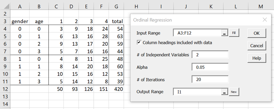
Figure 1 – Ordinal Regression dialog box

Press Ctrl-m and choose the Ordinal Regression option from the Reg tab (or from the Regression dialog box if using the older user interface). Now, fill in the dialog box as shown on the right side of Figure 1. After pressing the OK button, the output shown in Figures 2 and 3 is displayed.

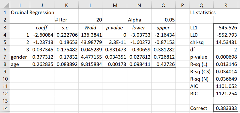
Figure 2 – Ordinal regression results (part 1)

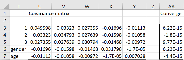
Figure 3 – Ordinal regression results (part 2)

The values near zero in column AA show that Newton’s method converged to a solution. The p-value of .0007 in cell R7 shows that the model is significantly different from the model without independent variables.

We see that this model predicts correctly 38.3% of the 420 observations; i.e. the observed category had the highest predicted probability 38.3% of the time (as opposed to ¼ = 25% based on pure chance).

The formulas shown in Figure 4 were used to produce the output in Figures 2 and 3.

Output	Range	Formula
Coefficients	I3:O8	=OLogitCoeff(A3:F11,4,TRUE,TRUE,O2,L2)
LL and related statistics	Q3:R12	=OlogitLL(A4:F11,J4:J8,4,TRUE)
Proportion correct	R14	=OlogitCorrect(A4:F11,J4:J8,4)
Covariance matrix	U3:Y7	=OlogitCov(A4:F11,J4:J8,4)
Convergence vector	AA3:AA7	=OlogitConverge(A4:F11,J4:J8,4)

Figure 4 – Key formulas

Raw Data Format

We can perform a similar analysis for data in raw format. When data is in raw format, then we have two choices. The first of these choices is to use the OLogitSummary array function to convert the data from raw format to summary format and then use the Ordinal Regression data analysis tool, using the summary data as input, as described above.

E.g. to convert the raw data in range A3:C13 of Figure 5 to summary format, we can use the array formula =OLogitSummary(A3:C13,TRUE), whose output is shown on the right side of Figure 5.

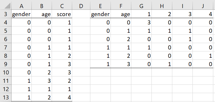
Figure 5 – Convert raw data to summary format

The other approach is to use the Ordinal Regression data analysis tool directly, using the raw data as input. Assuming that the data on the left side of Figure 5 represents only the first 10 of 420 rows of data equivalent to the summary data for Example 1 shown on the left side of Figure 1, we would follow the procedure described above, except that we would instead insert the range A3:C423 (from Figure 5, where the remaining 410 rows are not displayed) in the Input Range field of the dialog box shown in Figure 1. When the OK button is pressed, the output would be identical to that shown in Figures 2 and 3.

Examples Workbook

Click here to download the Excel workbook with the examples described on this webpage.

References

Agresti, A. (2013) Modeling Ordinal Categorical Data tutorial
http://statmath.wu.ac.at/research/talks/resources/slidesagresti_ordinal.pdf

Hyun Sun Kim (2004) Topics in ordinal logistic regression and its applications. Dissertation Texas A & M
https://core.ac.uk/reader/4268580