Basic Concepts
In a sample taken from a population, the kth order statistic is the kth smallest element in the sample. Suppose that the population has a discrete distribution with pdf f(z) and cdf F(z). First, we describe the (cumulative) distribution Fk(x) of the kth order statistic in a sample of size n taken from the population.
We assume that the population is {0, 1, 2, …}.
Cdf and Pdf Properties
Property 1: The cdf of the kth order statistic in the sample is
![]()
Proof:
![]()
![]()
Observation: Property 1 is based on the binomial distribution. The following is an equivalent version of the cdf based on the negative binomial distribution:
![]()
We also note that if G(x) is the cdf of the beta distribution Bet(k, n-k+1), then
![]()
Property 2: The pdf of the kth order statistic in the sample for x ≥ 0 is
![]()
Proof:
![]()
Pdf and Cdf Example
Example 1: Calculate the probability that the 2nd order statistic for a sample of size 8 from the Poisson distribution with mean 5 is less than or equal to 3 (i.e. the cdf at 3). Also, what is the pdf at 3?
Figure 1 shows four ways of calculating this value, namely 66.9%, as shown in cells D11, F12, I2 and I4.
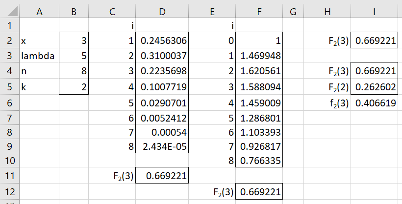
Figure 1 – cdf and pdf for 2nd order statistic
The formula in D11 is =SUM(D3:D9), where cell D3 contains the formula
=COMBIN($B$4,C2)*(1-POISSON.DIST($B$2,$B$3,TRUE))^($B$4-C2)*POISSON.DIST($B$2,$B$3,TRUE)^C2
The formula in cell F12 is =SUM(F2:F8)*POISSON(B2,B3,TRUE)^B5, where cell F2 contains the formula
=COMBIN($B$5+E2-1,$B$5-1)*(1-POISSON.DIST($B$2,$B$3,TRUE))^E2
Cell I2 contains the formula
=BETA.DIST(POISSON.DIST(B2,B3,TRUE),B5,B4-B5+1,TRUE)
Cell I4 contains the formula =ORDER_DIST(B2,B5,B4,TRUE,”poisson”,B3)
Note too that cell I5 contains the formula
=ORDER_DIST(B2-1,B5,B4,TRUE,”poisson”,B3)
and so the pdf at 3 is 40.66% as shown in cell I6 using the formula =I4-I5.
Expected Value
For a discrete distribution, the expected value of the kth order statistic for a sample of size n is
![]()
The following is an alternative way of expressing the expected value of the kth order statistic for a discrete population.
Property 3: The expected value of the kth order statistic for a sample of size n is
![]()
Proof: First observe that
![]()
![]()
![]()
Thus, for any m > 0
![]()
![]()
![]()
As m → ∞, mP(x(k) > m) → 0, and so
![]()
Observation: The expected values of the first and last order statistics are therefore
![]()
![]()
Expected Value Example
Example 2: Find the expected value of the 2nd order statistic for a sample of size 8 from a Poisson distribution with a mean of 5.
Figure 2 shows four ways of calculating the expected value, with the results shown in cells L2, L7, Q19 and T19.
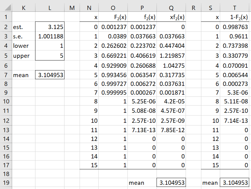
Figure 2 – Expected value of 2nd-order statistic
The value of 3.083 (cell L2) is based on a simulation of 1,000 samples using the Real Statistics formula =ORDER_SIM(B5,B4,TRUE,,,”poisson”,B3). See Confidence Intervals for Order Statistics, Medians and Percentiles for more information about the ORDER_SIM function. We see that the standard error for this estimate is a little over 1 with a 95% confidence interval of [1, 5].
Cell L7 contains the estimate of 3.10495 from the =ORDER_MEAN(B5,B4,,”poisson”,B3) formula. See Distribution of Order Statistics from a Continuous Population for more information about the ORDER_MEAN function.
We can see from column Q of Figure 2 that for x > 11, fk(x) = 0 and so we only need to sum between x = 0 and x = 11 to obtain the value shown in cell Q19. Note that cell O3 contains the formula =ORDER_DIST(N3,$B$5,$B$4,TRUE,”poisson”,$B$3). Cells P3, Q3 and Q19 contain the formulas =O3-O2, =N3*P3 and =SUM(Q2:Q17), respectively.
Finally, we can obtain the same value for the expected kth order statistic by using Property 3, as shown in cell T19. Note that cell T3 contains the formula
=1-ORDER_DIST(S3,$B$5,$B$4,TRUE,”poisson”,$B$3)
and cell T19 contains the formula =SUM(T2:T17).
Property 4: The variance of the kth order statistic for a sample of size n is
![]()
Real Statistics Support
The ORDER_DIST and ORDER_MEAN functions described in Order Statistics from a Continuous Population also support discrete populations.
Examples Workbook
Click here to download the Excel workbook with the examples described on this webpage.
References
David, H. A. and Nagaraja, H. N. (2003) Order statistics. Wiley
https://books.google.it/books/about/Order_Statistics.html?id=3Ts1yDLWXmQC&redir_esc=y
Omondi, O. C. (2016) Order statistics of uniform, logistic and exponential distributions
http://erepository.uonbi.ac.ke/bitstream/handle/11295/97307/MSc_Project2016.pdf?sequence=1&isAllowed=y
Arnold, B. C., Balakrishnan, N., Nagaraja, H. N. (2003) A First course in order statistics. Society for Industrial and Applied Mathematics
https://books.google.it/books/about/A_First_Course_in_Order_Statistics.html?id=gUD-S8USlDwC&redir_esc=y