Joint and Range Distribution from a Discrete Population

Joint Probability Properties

Property 1: Let F_j,k(x,y) be the joint distribution function for the j^th and k^th order statistic for a sample of size n taken from a discrete population with cdf F(x). Then for x < y

and for y ≤ x

Proof: For x < y

For x ≥ y

Property 2: Let f_j,k(x,y) be the joint pdf for the j^th and k^th order statistic for a sample of size n taken from a discrete population with cdf F(x) and pdf f(x). Then for x < y

and f_j,k(x,y) = 0 for x ≥ y.

Range Properties

Property 3: The pdf of the range statistic x_(n) – x₍₁₎ when w = 0 is

where f(x) is the pdf of the discrete population distribution. When w > 0 of the pdf of the range statistic x_(n) – x₍₁₎ is

where

where F(x) is the cdf of the discrete population distribution.

Observation: The cdf G(w) of the range statistic x_(n) – x₍₁₎ is therefore

where g(u) is the pdf as described in Property 3.

Property 4: The expected value of the range statistic x_(n) – x₍₁₎ is

Simulation Example

Example 1: Use simulation to estimate the probability that the range statistic for a sample of size 8 from the Poisson distribution with mean 5 is equal to 7 (i.e. the pdf at 7). Also, what is the cdf at 7?

The estimated pdf using simulation is .1773 and the cdf is .7625, as shown in Figure 1. These estimates were made by first creating 10,000 samples of size 8 (the rows in the range E2:L10001) from the desired Poisson distribution (only the first 10 rows are displayed in Figure 1). We can do this in Excel by inserting the formula =POISSON_INV(RAND(),B3) in every cell in range E2:L10001.

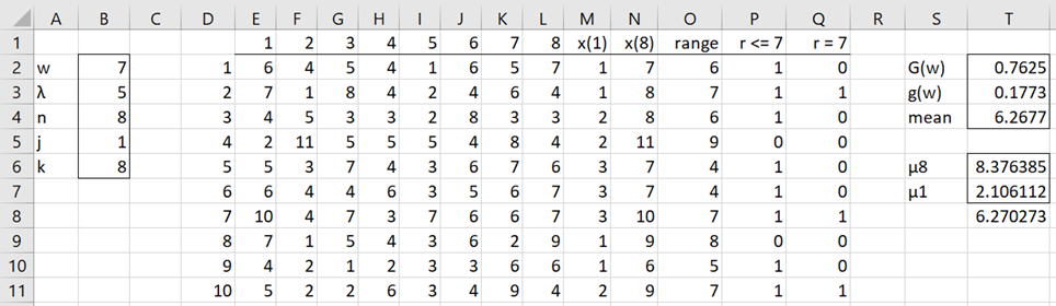
Figure 1 – Range statistic for the Poisson distribution: pdf and cdf

For each row in this range, we then compute the values of x₍₁₎, x₍₈₎ and the corresponding range. E.g. for the first row of simulated data, this is accomplished by placing the formulas =SMALL($E$2:$L$10001,B$5) in cell M2, =SMALL($E$2:$L$10001,B$6) in cell N2 and =N2-M2 in cell O2.

For each row, we now determine whether the range for that row meets the criteria range <= 7. This is done by placing the formula =IF(O2<=B$2,1,0) in cell P2. We can then highlight the range P2:P10001 and press Ctrl-D to fill in column P. The percentage of entries in this column that take the value 1 is a reasonable estimate of the cdf G(7) at w = 7. This is shown in cell T2 using the formula =AVERAGE(P2:P10001).

Pdf

We can calculate the pdf in a similar way. This time we place the formula =IF(O2=B$2,1,0) in cell Q2 (and similarly for the other cells in column Q) and then use the formula =AVERAGE(Q2:Q10001) in cell T3 to produce the estimate g(7) = .1773.

Note that before calculating the values in the cells in the columns to the right of column L, we first highlight range E2:L10001 and then copy the range using Ctrl-C and then paste values over the same range. The paste can be accomplished by clicking on Home > Clipboard|Paste > V (or by pressing the key sequence Alt-H-V-V. If this is not done, the SMALL function gets confused (at least this is what happened on my computer).

Note that this approach works to estimate the pdf and cdf for x_(k) – x_(j) for other values of j and k.

Other Examples

Example 2: Repeat Example 1 using Property 3.

Figure 2 shows how to perform this calculation, arriving at the pdf g(7) = .181832 (cell AE24), a little higher than the estimate calculated in Example 1.

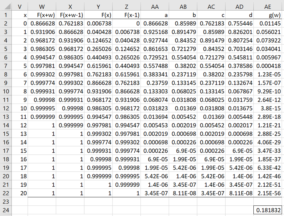
Figure 2 – Calculation of the pdf using Property 3

For example, for row corresponding to x = 1 (i.e. row 3), cell W3 contains the formula =POISSON.DIST(V3+$B$2,$B$3,TRUE), cell X3 contains the formula =W2, cell Y3 contains =POISSON.DIST(V3,$B$3,TRUE) and cell Z3 contains =Y2. The formulas for the other cells in columns W through Z are the same with one exception, namely the formula in cell Z2. This cell is supposed to contain the value of F(-1), which is assumed to be zero. Since =POISSON.DIST(-1,B3,TRUE) will yield an error value, we simply place 0 in cell Z2.

The values in columns AA, AB, AC, and AD are those for a, b, c, and d in Property 3. E.g. the formula in cell AA3 is =W3-Z3. The formula in cell AE4 is =AA3^B$4-AB3^B$4-AC3^B$4+AD3^B$4. Finally, cell AE24 contains the formula =SUM(AE2:AE22).

In the same way, we can calculate the values of g(0), g(1), …, g(7). The cdf G(7) is the sum of these values.

Range Examples

Example 3: Use the Real Statistics RANGE_DIST to estimate the probability that the range statistic for a sample of size 8 from the Poisson distribution with mean 5 is equal to 7 (i.e. the pdf at 7). Also, what is the cdf at 7?

The pdf can be calculated using the formula

=RANGE_DIST(B2,1,8,B4FALSE,”poisson”,B3)

The cdf can be calculated by the same formula with FALSE replaced by TRUE.

Figure 3 shows the values for g(w) and G(w) for different values of w.

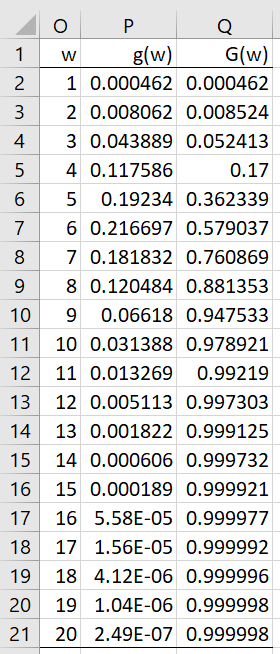
Figure 3 – pdf and cdf for range statistic

We see the results for w = 7 in row 8.

Example 4: Find the expected value of the range statistic for a sample of size 8 from a Poisson distribution with a mean of 7.

By Property 4, we see that the expected value of the range statistic is 6.270273 as shown in cell T8 of Figure 1. This is calculated by μ₈ – μ₁. This value is similar to the 6.2677 estimate in cell T4 based on the simulation described for Example 1. This estimate is calculated by the formula =AVERAGE(O2:O10001).

Real Statistics Support

The ORDER2_DIST function described in Joint and Range Distribution from a Continuous Population doesn’t currently support joint distributions from a discrete population. The RANGE_DIST function described on the same webpage also supports the range statistic μ_n – μ₁ from a discrete population, but not μ_k – μ_j for any j and k.

Examples Workbook

Click here to download the Excel workbook with the examples described on this webpage.

References

David, H. A. and Nagaraja, H. N. (2003) Order statistics. Wiley
https://books.google.it/books/about/Order_Statistics.html?id=3Ts1yDLWXmQC&redir_esc=y

Omondi, O. C. (2016) Order statistics of uniform, logistic and exponential distributions
http://erepository.uonbi.ac.ke/bitstream/handle/11295/97307/MSc_Project2016.pdf?sequence=1&isAllowed=y

Arnold, B. C., Balakrishnan, N., Nagaraja, H. N. (2003) A First course in order statistics. Society for Industrial and Applied Mathematics
https://books.google.it/books/about/A_First_Course_in_Order_Statistics.html?id=gUD-S8USlDwC&redir_esc=y