Objective
Our goal is to obtain a polynomial regression model of order k such that
We can accomplish this by using orthogonal contrast coefficients
where pj(x) is a polynomial of degree j. If we have a factor with t treatment levels, then k = t-1. Actually, we only include the pj(x) terms for which the jth trend is significant, as described in Trend Analysis. Furthermore, we will restrict ourselves to k ≤ 5 (i.e. linear, quadratic, cubic, quartic, or quintic). When these treatment levels are spaced equally with distance d, we will use the following polynomials where z = (x – x̄) / d.
Note that we need to use the lambda values from Figure 1 of Trend Analysis.
We also define the αj coefficients by
For the constant term α0, we use the coefficients cj = 1 for all j, and so
We also assume that λ0 = 1.
Example
Example 1: Create a polynomial regression model for Example 1 of Trend Analysis.
We first construct the tables shown in Figure 1.
Figure 1 – Polynomial regression model
Most of the information in the figure comes from Figures 3 and 4. The alpha coefficients in range I5:I9 are calculated as described above. E.g. cell I7 contains the array formula =SUMPRODUCT(B$2:F$2,B7:F7)/SUMSQ(B7:F7). The lambda values come from Figure 1. We see that z = (x – x̄)/d = (x–16.9)/5. Since the cubic and quartic trends are not significant, we can ignore these terms. Thus, our regression model is

Thus, the regression model is
Chart
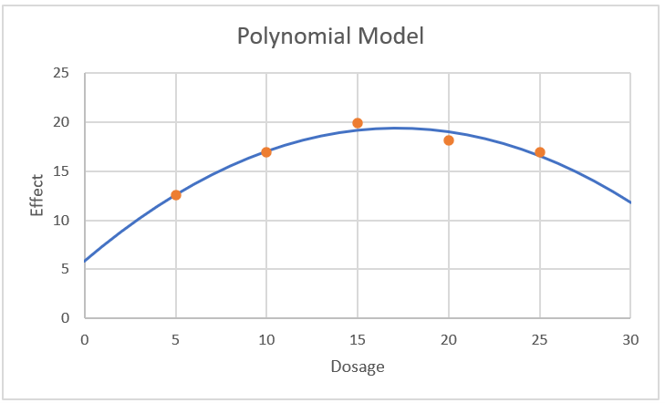
Figure 2 shows the graph of this model along with the five group means. Note that this graph is similar to that shown in Figure 5 in Trend Analysis.
Figure 2 – Chart of polynomial regression model
From the chart, we see that the dosage that yields the maximum effectiveness is somewhere between 15 and 20 (actually at 17.163).
Examples Workbook
Click here to download the Excel workbook with the examples described on this webpage.
References
Bergerud, W. (1988) Determining polynomial contrast coefficients. Biometrics Information
No longer available online
Penn State University (2021) Orthogonal polynomials
https://online.stat.psu.edu/stat502/lesson/10/10.2
Howell, D. C. (2010) Statistical methods for psychology (7th ed.). Wadsworth, Cengage Learning.
https://labs.la.utexas.edu/gilden/files/2016/05/Statistics-Text.pdf
Fisher, R. A., Yates, F. (1963) Statistical tables, 6th ed. Macmillan Publishing
https://digital.library.adelaide.edu.au/dspace/bitstream/2440/10701/1/stat_tab.pdf
Anderson, R. L. (1942) Tables of orthogonal polynomial values extended to N=104
https://babel.hathitrust.org/cgi/pt?id=coo.31924000087100&seq=10
Horsley, R. (2022) Orthogonal polynomial contrasts individual df comparisons> equally spaced treatments.
No longer found online


