Objective
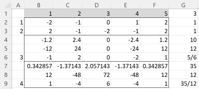
We can use the equations for linear, quadratic, cubic, quartic, and quintic trends to calculate the coefficients in the table shown in Figure 1 of Trend Analysis.
Example
We now illustrate this process in Figure 1 for the case where there are 5 groups.
Figure 1 – Coefficients for equal intervals
Explanation
We start with the values 1, 2, 3, 4, 5, as shown in row 1. The average x̄ = 3 (cell G3). Here t = 5 (cell F1) and d = 1.
To calculate the linear coefficients, we place the formula =B1-$G3 in cell B2, highlight range B2:F2, and press Ctrl-R. Since the coefficients in row 2 are integers with no common divisor, λ1 = 1 (cell G2).
To calculate the quadratic coefficients, we place the formula =B2^2-($F1^2-1)/12 in cell B3, highlight range B3:F3, and press Ctrl-R. Since the coefficients in row 3 are integers with no common divisor, λ2 = 1 (cell G3).
To calculate the cubic coefficients, we place the formula =B2^3-B2*(3*$F1^2-7)/20 in cell B4, highlight range B4:F4, and press Ctrl-R. This time, we see that the values in row 4 are not integers, but if we multiply all the values in row 4 by 10, we obtain integer values as shown in row 5. Since 12 is a common factor for all the values in row 5, we now divide these values by 12 to obtain the described coefficients as shown in row 6. Note that we multiplied the row values by 10 and then divided them by 12, λ3 = 10/12 = 5/6 (cell G6).
To calculate the quartic coefficients, we place the formula =B2^4-B2^2*(3*$F1^2-13)/14+3*($F1^2-1)*($F1^2-9)/560 in cell B7, highlight range B7:F7 and press Ctrl-R. The values in row 7 are not integers, but it is less obvious what we need to multiply these values by to obtain integers. It turns out that if we multiply by 35 and divide by 12, we get the desired quartic coefficients as shown in row 9. Thus, λ4 = 35/12 (cell G9).
Real Statistic Support
Real Statistic Function: The Real Statistic Resource Pack provides the following worksheet function.
TREND_COEFF(k, lambda): returns the coefficient matrix for a treatment with k equally spaced groups for k ≥ 2.
For k = 2, 3, 4, 5, 6, the matrix that is returned has k-1 rows and k columns. For k ≥ 7, the matrix has 5 rows and k columns (i.e. only linear, quadratic, cubic, quartic, and quintic coefficients are returned).
If lambda = TRUE (default FALSE), then an extra column is appended to the right side of the output with the lambda values.
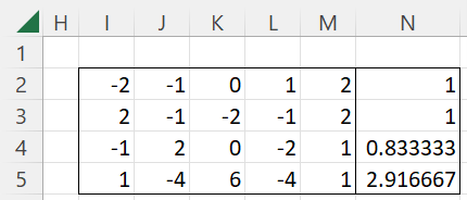
For Example 1, we can use the array formula =TREND_COEFF(5,TRUE) to obtain the results shown in Figure 2.
Figure 2 – TREND_COEFF(5, TRUE)
Examples Workbook
Click here to download the Excel workbook with the examples described on this webpage.
References
Bergerud, W. (1988) Determining polynomial contrast coefficients. Biometrics Information
No longer available online
Penn State University (2021) Orthogonal polynomials
https://online.stat.psu.edu/stat502/lesson/10/10.2
Howell, D. C. (2010) Statistical methods for psychology (7th ed.). Wadsworth, Cengage Learning.
https://labs.la.utexas.edu/gilden/files/2016/05/Statistics-Text.pdf
Fisher, R. A., Yates, F. (1963) Statistical tables, 6th ed. Macmillan Publishing
https://onlinelibrary.wiley.com/doi/abs/10.1002/bimj.19710130413
Anderson, R. L. (1942) Tables of orthogonal polynomial values extended to N=104
https://babel.hathitrust.org/cgi/pt?id=coo.31924000087100&seq=10
Horsley, R. (2022) Orthogonal polynomial contrasts individual df comparisons: equally spaced treatments.
No longer found online

