Basic Concepts
The Siegel-Tukey test (for equal variability) is a nonparametric test to determine whether two samples come from populations with equal variances. When data is clearly normally distributed, a parametric test is preferred.
Assumptions:
- The two (random) samples are independent
- The data is at least ordinal
- The two populations have the same medians
If the population medians are known but unequal, then the data can be adjusted to satisfy this last assumption. If the population medians are not equal and are unknown, then even when the sample medians are equal, there is no guarantee this test will be valid.
Suppose the median of the population corresponding to sample 1 is m1 and the median of the population corresponding to sample 2 is m2. Suppose further that m1 < m2, then we can subtract m2 – m1 from all the elements in sample 2 to satisfy assumption #3. Alternatively, we can add m2 – m1 to all the elements in sample 1.
Example
Example 1: Two drugs are known to be equally effective (i.e. they have the same mean or median). Based on the data in Figure 1, use the Siegel-Tukey test to determine whether the two populations have the same variability.
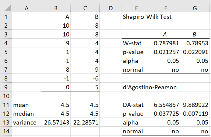
Figure 1 – Siegel-Tukey test data
We see from the right side of the figure that the samples are not normally distributed, and so the usual F-test may not be appropriate.
The null hypothesis is that the populations from which the samples are taken have equal variances.
When the null hypothesis is true, the average ranks of the two samples should be equal (when combined ranks are used). Here, ranks are determined based on the data value’s distance from the median, as explained next.
Methodology
First, we combine the data in B2:C9 into a single sample as shown in columns I and J of Figure 2.
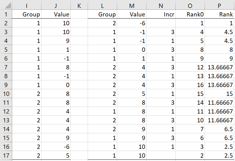
Figure 2 – Siegel-Tukey rankings
We next sort this data as shown in columns L and M. This can be done by placing the Real Statistics array formula =QSORTRows(I2:J17,2) in range L2:M17 (see Sorting and Removing Duplicates by Rows). Alternatively, you can use Excel sorting capability (Data > Sort & Filter|Sort) in Sorting and Filtering. Excel 365 and 2021 users can also use SORT(I2:J17,2) (Sorting and Filtering Functions).
Ranking
We now create the initial rankings, as shown in column O. The rank of the smallest value (cell M2) is set to 1 (cell O2). The rank of the largest value (cell M17) is set to 2 (cell O17). The value before this one (cell M16) is set to 3 (cell O16). Next, the rank of the second-to-smallest value (cell M3) is set to 4 (cell O3), followed by a rank of 5 (cell O4) for the next smallest value (M4). After that, we rank the next two high values (in rows 14 and 15). We continue in this way, alternating between low and high values until all the elements are ranked.
We can do this in Excel by placing alternating 1’s and 3’s in column N. Then, after placing 1 in cell O2 and 2 in cell O17, we place the formula =O2+N3 in cell O3, highlight range O3:O9, and press Ctrl-D. Similarly, we place the formula =N10+O11 in cell O10, highlight range O10:O16, and press Ctrl-D.
We observe that although cells M16 and M17 have the same value, they have different ranks (2 and 3). To fix this, we replace these ranks with their average of such ranks, as shown in cells P16 and P17. Similarly, cells M11, M12, and M13 contain the same value, and so we replace their ranks by the average of these ranks, namely (14+11+10)/3 = 35/3 = 11 2/3, as shown in cells P11, P12, and P13.
We can accomplish this in Excel by placing the formula =AVERAGE(IF(M$2:M$17=M2,O$2:O$17,””)) in cell P2, highlighting range P2:P17, and pressing Ctrl-D.
Mann-Whitney test
Now that we have calculated the appropriate rankings, we use the Mann-Whitney test procedure with these rankings, as shown in Figure 3.
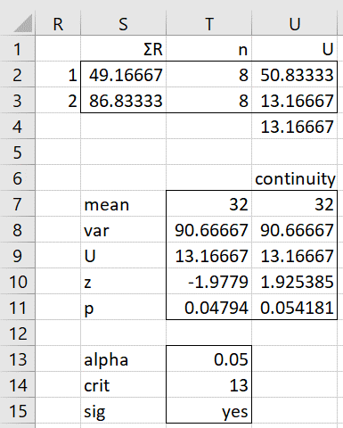
Figure 3 – Calculating the test significance
We calculate R1 (cell S2) by summing all the values in column P that correspond to a 1 in column L. Similarly, we calculate R2 (cell S3) by summing all the values in column P that correspond to a 2 in column L. We then calculate U1 and U2 (cells U2 and U3) via the formulas
Ui = n1n2 + ni(ni+1)/2 – Ri
U is then the minimum of U1 and U2.
We do this in Excel by placing the formula =SUMIF(L$2:L$17,R2,P$2:P$17) in cell S2, =COUNTIF(L$2:L$17,R2) in cell T2, and =T$2*T$3+T2*(T2+1)/2-S2 in cell U2. We then highlight range S2:U3, and press Ctrl-D. U is calculated in cell U4 by the formula =MIN(U2,U3).
We calculate the p-value using the normal approximation for the Mann-Whitney test as shown in range S7:T10, arriving at a p-value of .04794 (two-tailed test), which indicates a significant result (if α = .05). We see, however, that if we use a continuity correction, then p-value = .054181 (cell U11), which indicates a non-significant result. Note that the formula used to calculate the z-statistic (cell U10) is =(ABS(U9-U7)-0.5)/SQRT(U8).
Actually, with such small samples, we can use the table of critical values (see Mann-Whitney Table). The critical value when α = .05 and n1 = n2 = 8 is 13. Since U = 13.16667 > 13 = U-crit, we have a non-significant result, indicating that we don’t have enough evidence to conclude that the population variances are different.
Worksheet Function
Real Statistics Function: The Real Statistics Resource Pack provides the following function for the data in R1 and R2.
ST_TEST(R1, R2, lab, tails, ties, cont): returns a column array with the values U, z, r effect size, and p-value.
R1 and R2 must be column arrays or ranges with no missing data. If lab = TRUE (default FALSE), a column of labels is appended to the output. tails = 1 or 2 (2 is the default). If ties = TRUE (default), then a ties correction will be applied. If cont = TRUE (default), then a continuity correction of .5 is applied.
We can use this function to get the results for Example 1, as shown in Figure 4.
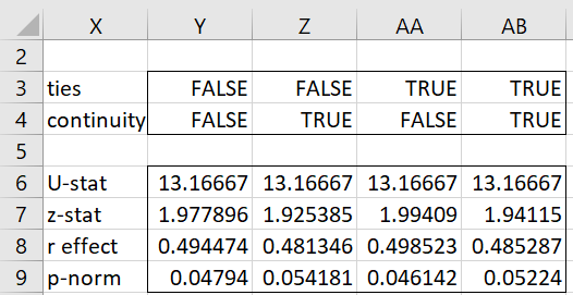
Figure 4 – Using the ST_TEST function
E.g. range X6:Y9 contains the formula =ST_TEST($B$2:$B$9,$C$2:$C$9,TRUE,2,Y3,Y4) and range AB6:AB9 contains the formula =ST_TEST($B$2:$B$9,$C$2:$C$9,FALSE,2,AB3,AB4)
Examples Workbook
Click here to download the Excel workbook with the examples described on this webpage.
Links
References
Siegel, S., Castellan, N. J. (1988) Nonparametric statistics for the behavioral sciences, 2nd ed.
https://psycnet.apa.org/record/1988-97307-000