Basic Concepts
We now present the permutation test for paired samples. This non-parametric test does not make assumptions about normality, homogeneity of variances, or the shape of the underlying distribution. For this test, the null hypothesis is
H0: any difference between the pairs in the two populations is due to chance.
We demonstrate how this test is conducted via the following example.
Example
Example 1: Suppose that a sample of nine identical twins is made where one of the twins selected at random is given treatment A and the other is given treatment B. Determine whether there is a significant difference between the treatments based on the data in Figure 1.
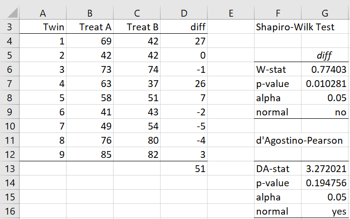
Figure 1 – Paired Samples Data
As for other paired tests, this test is equivalent to a test on one sample consisting of the differences between the pairs (as shown in column D). The sum of these differences is 51, as shown in cell D13. We see from the Shapiro-Wilk test that this data set is not normally distributed (although the conclusion is different from the d’Agostino-Pearson test), and so we decide to use the Paired Permutation test.
Approach
If the null hypothesis is true, then it doesn’t matter which twin receives Treatment A and which receives Treatment B. If, for example, for Twin 1 we flip the treatments, then diff would be -27 instead of 27. Essentially, this is like flipping a coin as to which twin gets which treatment. Thus, there are 29 = 512 possible orderings of the signs of the elements in column D.
Actually, since diff = 0 for Twin 2, we can exclude this twin from the analysis. It turns out that we would get the same result even if we retain this value, except that the processing time would be slower. Now, there are 28 = 256 possible orderings. These are shown in Figure 2.
Row 2 contains the absolute values of the eight difference values in column D of Figure 1 (excluding the zero value for Twin 2). Rows 3 through 258 of Figure 2 contain the 256 permutations, along with the sums (in column W).
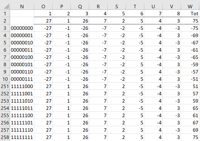
Figure 2 – Permutations
Generating the permutations
Figure 2 displays the first 8 permutations in the list and the last 8 permutations. The middle 256-16 = 240 permutations are not displayed. The various permutations are determined by the values in column N. E.g. the value 00000101 in cell N8 indicates that a negative sign should be assigned to the first 5 values as well as the 7th value in row 2, and a positive sign should be used for the 6th and 8th values. A “0” in “00000101” indicates a “-“ sign, while a 1 indicates a “+” sign.
We obtain the values in Figure 1 by inserting the Real Statistics formula =INIT_PARTITION(8) in cell N3 and =NEXT_PARTITION(N3) in cell N4 (see Guttman Reliability). Next, we highlight the range N4:N258, and press Ctrl-D. We also insert the formula =O$2*(2*MID($N3,O$1,1)-1) in cell O3, highlight range O3:V3, and press Crtl-R. Finally, we insert the formula =SUM(O3:V3) in cell W3, highlight range O3:W258, and press Ctrl-D.
Obtaining the p-value
To obtain the p-value for this test, we need to determine what percentage of the totals in column W are at least as large as the total of 51 (cell D13) for observed differences shown in Figure 1. This yields the p-value for the one-sided test for the right tail. We obtain this value via the formula =COUNTIF(W3:W258,”>=”&D13)/2^V1. This yields a p-value of 39/256 = .152344.
For the two-tailed test, we simply double this value to obtain a p-value of .304688.
Note that the list of permutations in Figure 2 is symmetric. We see that the last total in column W is the negative of the first total in column W. Similarly, the second-to-last total is the negative of the second total. Etc. This means that we only need to generate the first half of the listing in Figure and use the absolute value of the value in column W. Thus, the one-tailed p-value can also be calculated via the formula =SUM(IF(ABS(W3:W130)>=D13,1,0)/2^V1).
Note that we would have liked to use the formula
=COUNTIF(ABS(W3:W130),”>=”&D13)/2^V1
but this is not a legal formula in Excel since the first argument of the COUNTIF function must be a range.
Worksheet Function
Real Statistics Function: The Real Statistics Resource Pack provides the following function.
PERM_TEST(R1, R2, tails) = the p-value of the paired sample permutation test for the data in arrays R1 and R2. tails = 2 (two-tailed test, default), 1 (one-tailed test), or -1 (one-tailed test with larger p-value)
R1 and R2 must be column arrays or ranges with the same number of rows and no missing data. R2 is optional. If it is omitted, then a one-sample permutation test is employed. R2 can also be replaced by a numeric value, in which case the one-sample test is performed on the values in R1 less this numeric value.
We obtain the one-tailed p-value of .152344 for Example 1 by using the formula =PERM_TEST(B4:B12,C4:C12,1). We get the same result by using the formula =PERM_TEST(D4:D12,,1) or =PERM_TEST(D4:D12,0,1). The two-tailed p-value can be calculated by =PERM_TEST(B4:B12,C4:C12) or =PERM_TEST(D4:D12).
One further note: The permutation test is quite resource intensive, and should only be used with relatively small samples. On my computer with a sample of around 20 pairs, the PERM_TEST is quite fast, but at about 25 pairs, it takes about a minute to generate the p-value, and beyond that, it starts to slow down quite quickly.
Examples Workbook
Click here to download the Excel workbook with the examples described on this webpage.
Links
Reference
Siegel, S., Castellan, N. J. (1988) Nonparametric statistics for the behavioral sciences, 2nd ed.
https://psycnet.apa.org/record/1988-97307-000