Objective
The objective of the Anderson-Darling test is similar to that of the Kolmogorov-Smirnov test, but it is more powerful. This is so since all the data values are considered, not just the one that produces the maximum difference. Also, more weight is given to the tails of the distribution being fitted. Generally, this test should be used instead of the Kolmogorov-Smirnov test. Unlike the version of the one-sample Kolmogorov test described on this website, the approach used varies based on the theoretical distribution being fitted.
How to Perform the Test
Suppose you want to see how well sample X fits a continuous distribution with cumulative distribution function (cdf) F(x). To perform the one-sample Anderson-Darling test, first sort the sample X in increasing order: x1 ≤ x2 ≤ … ≤ xn and then calculate the following statistic

Specified Parameters
We start with a distribution function F(x) that is fully determined (i.e. none of the parameters need to be estimated from the sample). Figure 1 displays the critical values in this case, at least for large samples, although usually, samples of size n > 7 will suffice. We will refer to such a distribution as generic or specified.
Figure 1 – Anderson-Darling critical values
As for the KS test, there is a significant difference between the sample data and the theoretical distribution, provided A ≥ c.
Actually, we can use the AD_DIST(x) and AD_INV(p) functions to obtain more accurate estimates of the critical values and p-values. Click here for details.
The critical values and p-values are also valid when the data is fitted to a uniform distribution between 0 and 1 (e.g. when determining whether the data is random).
Estimated Parameters
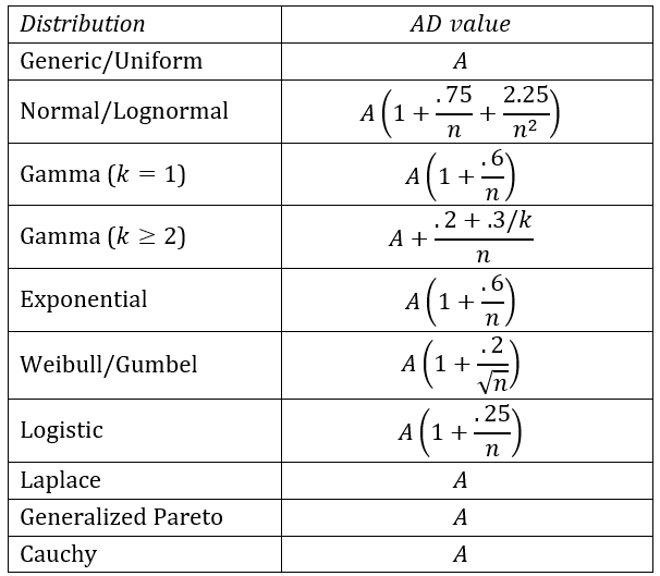
When the parameters of the distribution are unknown but need to be estimated from the sample, we need to perform a few additional steps. First, we calculate the test statistic AD based on A, but which may be modified depending on the specific distribution, as described in Figure 2.
Figure 2 – Anderson-Darling test statistic
For the gamma distribution, k is the shape parameter, referred to as α in Gamma Distribution.
We determine that there is a significant difference between the sample data and the theoretical distribution provided AD ≥ crit, where crit is the critical value (for a given value of α) defined based on the table of critical values shown in Anderson-Darling Statistical Table.
Normal Distribution
Note that for the normal distribution, the critical value is given by
where a, b, and d are shown in the table of critical values shown in Anderson-Darling Statistical Table.
For the normal distribution, p-values can be obtained from Figure 3.
| AD | p-value |
| AD ≤ .2 | 1 – exp(-13.436 + 101.14 AD – 223.73 AD2) |
| .2 < AD ≤ .34 | 1 – exp(-8.318 + 42.796 AD – 59.938 AD2) |
| .34 < AD < .6 | exp(0.9177 – 4.279 AD – 1.38 AD2) |
| AD ≥ .6 | exp(1.2937 – 5.709 AD + 0.0186 AD2) |
Figure 3 – p-values for normal distribution
Example
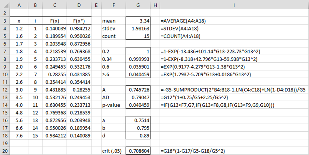
Example 1: Repeat Example 2 of Kolmogorov-Smirnov Test for Normality using the Anderson-Darling test for normality (the data is repeated in range A4:A18 of Figure 4).
Figure 4 – Anderson-Darling test for normality
We insert the formula =NORM.DIST(A4,$G$3,$G$4,TRUE) in cell C4 and the formula =LARGE($C$4:$C$18,B4) in cell D4. Then we highlight range C4:D18 and press Ctrl-D. The Anderson-Darling A statistic is displayed in cell G12, and the modified version AD is shown in cell G13. The p-value (cell G14) is calculated as described in Figure 3 (using range G7:G10). Finally, the critical value (cell G20) is calculated using the a, b, and d critical values from the table of critical values in Anderson-Darling Statistical Table.
Note that p-value = .040459, and so we conclude that the data is significantly different from normality. This result is similar to the p-value = .043227 that we obtained from the Shapiro-Wilk test in Example 2 of Shapiro-Wilk Test.
Note too that the same test can be used for the lognormal distribution. For data {x1, …, xn}, you simply test {ln x1, …, ln xn} for a fit with the normal distribution.
Worksheet Functions
Real Statistics Functions: The following functions are provided in the Real Statistics Pack:
ANDERSON(R1, dist, k) = the Anderson-Darling AD statistic for the theoretical cdf values in range R1 (assumed to be sorted in ascending order) based on the distribution defined by dist.
ADCRIT(n, alpha, dist, k, interp) = the critical value for the Anderson-Darling test for the distribution specified by dist.
ADPROB(x, dist, k, iter, interp, txt) = an approximate p-value for the Anderson-Darling test at x (which is set to the AD statistic) for the specified distribution, based on an interpolation of the critical values in the table in Anderson-Darling Statistical Table, using iter number of iterations (default = 40) to calculate the approximation.
ADTEST(R1, dist, lab, iter, alpha): returns an array with the Anderson-Darling D statistic, the critical value, and the estimated p-value for the Anderson-Darling test on the data in range R1 (not necessarily in sorted order) based on the stated distribution dist.
Function arguments
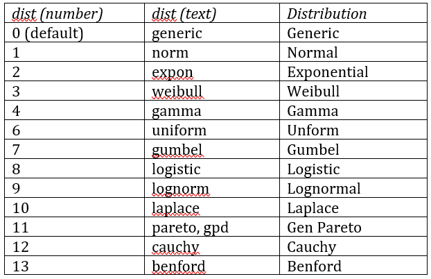
The dist parameter takes the values shown in Figure 5.
Figure 5 – dist values
n is the sample size. This value must be supplied for the normal, lognormal, Laplace, Cauchy, and Generalized Pareto distributions. It is ignored, and can be omitted for the other distributions. For the Laplace or Generalized Pareto distributions, n must take a value ≥ 10 (and ≤ 100 for the GPD). For the Cauchy distribution, n must take a value ≥ 5.
k = the shape parameter (alpha) of the gamma distribution (default 1), and is ignored for the other distributions, with the following exception. k is also used in the ADPROB function for the Laplace, Cauchy, and Generalized Pareto distributions where k = the sample size, which must take a value in the ranges described for n above,
alpha is the significance level (default .05). If interp = TRUE then harmonic interpolation is used in calculating the critical value; otherwise, linear interpolation is used. If lab = TRUE (default FALSE), then an extra column of labels is appended to the output from ADTEST to yield a 3 × 2 range.
As described earlier on this webpage, the Anderson-Darling test statistic requires the calculation of the natural log. If the log of zero or a negative number is required, then the ANDERSON and ATEST functions will return an error value.
Alpha ranges
Note that the values for α in the table of critical values in Anderson-Darling Statistical Table range from .01 to .15 for the generic distribution, from .0025 to .25 for the exponential distribution, from .005 to .25 for the gamma distribution, from .005 to .20 for the normal distribution, and from .01 to .25 for the other distributions.
When txt = FALSE (default) for values of x smaller than the lower limit, the value of =ADPROB(x, n, dist, k, iter, interp) is artificially set to 0, and for values of x bigger than the upper limit, the value of this formula is set to 1. When txt = TRUE, the output takes a form such as “< .01” or “> .25”.
Arguments for the ADTEST function
For ADTEST, dist and alpha are as described above. ADTEST returns a column array with the values AD statistic, p-value, and critical value. If lab = TRUE (default FALSE), then a column of labels is appended to the output.
R1 is a column array or range that contains the sample data. The exception is the generic case, where R1 contains the theoretical cdf values. Note that for the uniform distribution, which is assumed to be on the interval (0,1), the sample and theoretical cdf values are the same.
For the ADTEST function for the Generalized Pareto distribution, the location parameter μ for the data in R1 must be zero (otherwise, you must subtract μ from all the sample data values).
iter argument for the ADTEST function
iter is used to determine the distribution parameters for the specified distribution (defined by dist). If iter > 0 then these parameters are estimated using the maximum likelihood estimate (MLE) based on the GAMMA_FIT, WEIBULL_FIT, etc. functions, using the default argument values except that the number of iterations is set to the iter value (see Distribution Fitting via the MLE).
If iter = 0 or -1, the distribution parameters are estimated using the method of moments based on the GAMMA_FITM, WEIBULL_FITM, etc. functions using the default argument values, except that if iter = -1, the pure argument is set to TRUE (see Distribution Fitting via the Method of Moments).
For the Cauchy distribution (dist = 12 or “cauchy”), if iter = 0, the trim mean estimate is used, while if iter = -1, the median estimate is used; in either case, the exclusive version of the IQR is used.
If iter = -2, then the distribution parameters are estimated by the WEIBULL_FITR and CAUCHY_FITX functions using the default arguments. In fact, iter = -2 is only used for the Weibull or Cauchy distributions.
Alternative form of the ADTEST function
Note that if the default WEIBULL_FIT, GAMMA_FITM, etc. argument values, as described above, don’t yield the desired result, you can separately estimate the distribution parameters and then use the following alternative version of the ADTEST function.
ADTEST(R1, dist, lab, , alpha, param1, param2)
If param1 is specified, then the value of iter is ignored, and the distribution parameter values are those specified by param1 and, if necessary, by param2. Note that this form can’t be used for dist = 0 or “specified”, or for dist = 6 or “uniform”. For the uniform distribution, the parameters are automatically set to 0 and 1. For the specified case, no parameters are used since R1 contains the theoretical cdf values, and so these don’t need to be estimated from the distribution parameters.
Normal Distribution with specific mean or variance
You can also use the Anderson-Darling Test to determine whether a data set fits a normal distribution with a specified mean or variance. The ANDERSON, ADCRIT, ADPROB, and ADTEST support this option when the dist argument takes one of the following values:
| dist (number) | dist (text) | description for ADTEST |
| 1.1 | norm-mean | mean based on sample; variance specified via param2 |
| 1.2 | norm-var | variance based on sample; mean specified via param1 |
The AD value (see Figure 2) is equal to A. The k argument is not used in the ANDERSON, ADCRIT, and ADPROB worksheet functions.
Alternative Analysis
For Example 1, the value in cell G13 can be computed by =ANDERSON(C4:C18,1). Note that the cell range corresponds to the F(x) values in column C, not the data values in column A.
Here, the F(x) values are based on the sample mean and standard deviation. If, instead, we wanted to test whether the data in range A4:A18 of Figure 4 was a good fit for a normal distribution with mean 4 and standard deviation 2, we would use the analysis shown in Figure 6.
Figure 6 – Anderson-Darling test for a generic distribution
Example using worksheet functions
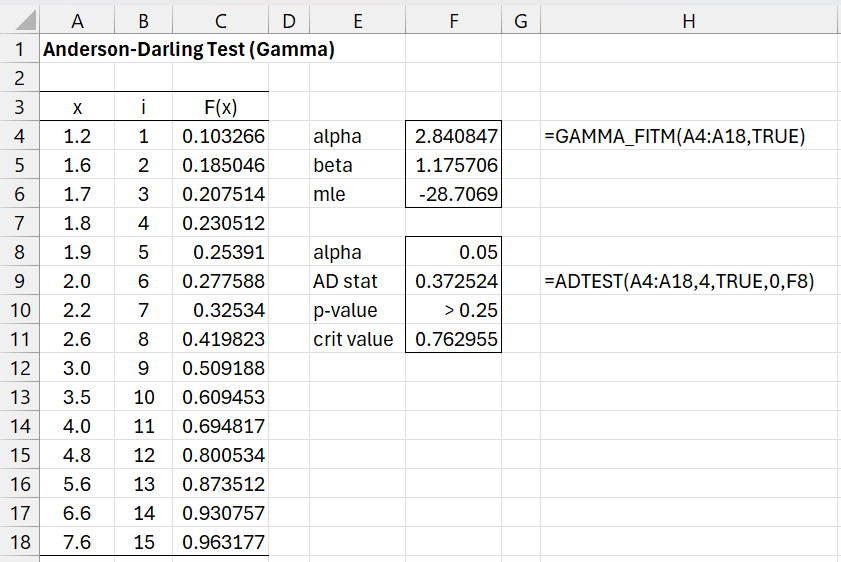
Example 2: Test whether the data in range A4:A18 of Figure 7 is a good fit for the gamma distribution.
Figure 7 – Anderson-Darling test for gamma distribution
This time, we use the ADTEST array function to compute the p-value for the test. Since p-value = “>.25”, we conclude that the gamma value is a good fit for the data. Note that p-value = “>.25” means that the calculated Anderson-Darling statistic (.3725) is less than the smallest value on the table of critical values, which in this case is .475 (when α = .25 for k = 3, the value in cell F4). Thus, we really know that p-value >> .25.
We would have gotten the same result for the p-value by using the formula =ADPROB(F9,4,F4). Note that this time, we need to explicitly refer to the k value in cell F4. We could have calculated the Anderson-Darling statistic by using the formula =ANDERSON(C4:C18,4,F4).
Note that while the ANDERSON function uses the theoretical F(x) values (column C), ADTEST uses the data values (column A). The only exception to this is for a test of a generic distribution (i.e. one where there are no unknown parameters). In this case, ADTEST must reference the theoretical F(x) values. E.g. to calculate the results shown in range F9:F11 of Figure 6, we could use the array formula =ADTEST(C4:C18,,TRUE).
Data Analysis Tool
You can also perform the One-sample Anderson-Darling Test via the Goodness-of-Fit data analysis tool. Click here for more information about this data analysis tool.
Examples Workbook
Click here to download the Excel workbook with the examples described on this webpage.
Links
References
Ang, A. H. and Tang, W. H. (2006) Probability Concepts in Engineering: Emphasis on Applications in Civil & Environmental Engineering
Pettitt, A.N. (1976) A two-sample Anderson-Darling rank statistic. Biometrika (1976) 63 (1): 161-168
https://www.jstor.org/stable/2335097?origin=crossref
Stephens, M.A. (1979) The Anderson-Darling statistic. Technical Report No. 39. Stanford University.
https://archive.org/details/DTIC_ADA079807/page/n19/mode/2up
Puig, P. and Stephens, M. A. (2000) Tests of fit for the Laplace distribution, with applications
Available from Researchgate


Hi Charles
For the AD values quoted in figure 2 which depend on the distribution being tested, how are these derived from first principles?
Hi Judith,
I believe these were developed via simulations. You can get more details from the references.
Charles
Hi Charles,
Are you planning on implementing the Anderson-Darling Test for partially known normal distributions (e.g. a normal distribution with mean 0 and unknown variance, or alternatively one with an unknown mean and known variance)? Thank you very much.
Regards,
Nelson
Hello Nelson,
I will try to add this capability in the next release.
Charles
Charles,
as far as I understood, we can’t do One-Sample AD Test for a Pareto dist with your add-in?
You have 8 distributions on your Figure. 5 which does not include Pareto Dist, right?
Anil,
That is correct. I don’t currently support a Pareto distribution for the one-sample AD test.
I plan to look into whether there is a version of the AD test that supports the Pareto distribution.
Charles
Dear Charles,
I am little confused as to how to calculate the p-value. On another page, you mention Marsaglia ADDIST approximation. Here you mention the ADPROB which is based on a piecewise valuation defined in Fig. 3 that comes from D’Agostino-Stephens. Which one does what?
Dear Gwenn,
They are two different ways of estimating the p-value. The estimates should be reasonably close.
ADPROB is based on interpolations between the table of critical values shown in
Anderson-Darling Statistical Table
AD_DIST uses the formulas shown at
Anderson Darling Distribution
Charles
Dear Charles,
I really appreciate your post, this is extremely useful! However, I have a question for you. Do you have the formulae (similar to the ones in Figure 3) to calculate the p-values for the rest of the distributions you mentioned in this post? And if so, could you share those please?
Warm regards from Mexio City,
Eduardo
Hello Eduardo,
Sorry, but I don’t. Yo calculate the p-values for the other distributions, I use interpolations from the critical values.
Charles
Hi Charles, it is possible to test anderson darling and at simultaneously get a p – value to pdf gamma. I have a sample of a generated series, and I also need to try adjusting it to a gamma pdf discriminating some data.
Sorry, I don’t understand your question.
Charles
Hi Charles,
If I want to test for Weibull distribution, can I still use the formula in figure 3 to find the p-value?
Thank you.
Hello Jessica,
No, that is only for the normal distribution. The webpage describes how to calculate the p/value for the Weibull distribution.
Charles
Hi Charles,
May I know which part mentioning about p-value for Weibull? Is it figure 2?
Thanks
Hello Jessica,
Use the ADPROB or ADTEST function.
Charles
Dear Charles,
First of all, thank you very much for this site. It is very helpful!
Secondly, how can I perform an Anderson-Darling test with censored data?
Thanks
Hi Rafael,
Glad that you find the site helpful.
Real Statistics doesn’t yet support this topic. The following paper may be helpful:
https://www.researchgate.net/publication/239182869_Nonparametric_Goodness-of-Fit_Tests_for_Censored_Data
Charles
Dear Charles,
Thanks for your quick answer. I will read the paper.
Hi Charles,
If have sample size more than 300 and I want to test if this set of data follows exponential distribution, can I still use Anderson-Darling test? or is there any better way to do it? Thanks
Jessica
Sorry, correction on my sample size. Sample size is 47.
Hello Jessica,
Yes, you can use Anderson-Darling test to determine whether data follows an exponential distribution.
Charles
Hi Charles,
This is to test normality in regards to what? I have a set of failure data that I expect to follow Weibull distribution. How can I use AD test to verify this?
Normality refers to the normal distribution. How to test whether the data fits with a Weibull ditribution is described on this webpage.
Charles
Hi Charles,
Could yu please check the p-value formula 0,34<D<0,6? I belive the correct one is =EXP(0,9177-4,279*D+1,38*D^2) instead of =EXP(0,9177-4,279*D-1,38*D^2). The formula seems to provide a better result if you add the term +1,38*D^2.
Hi Allan,
All the references that I have seen use the formula =EXP(0,9177-4,279*D-1,38*D^2). Can you give me a reference where the other formula is used?
Charles
Hi Charles,
Could you please check that the formula for the A statistic is correct? Instead of a difference between the two LN() parts of the equation, a few other references show this as an addition. The formula seems to give a better result if the two terms are added!
Thanks for providing a great website.
Best regards
Hi Mark,
Yes, you are correct. I believe that this is a typing mistake and that all the calculations on the website and in the Real Statistics software used the correct formula.
I have now corrected the formula on the webpage. Thank you very much for identifying this error and improving the accuracy of the website.
Charles
Charles,
Your Real Statistics Add-In Package, not to mention your comprehensive website is second to none!!
I was running a One-Sample Anderson Darling test. In order to ensure my understanding, I worked through your Example 1 …with the 15 data points and a normal distribution. When I work through the example on the web page, I match your answers perfectly. However, when I run the same problem on the Goodness of Test function in the Real Statistics Data Pack, I get a p-value of .0329 instead of .040459 as depicted in your example. It so happens if I use stdev.p instead of stdev.s I match the .0329. Would appreciate your help. Thanks, Jeff
Hello Jeff,
If on the data analysis tool you choose the MLE or Pure Moments option, then you will get the .0329 value (using stdev.p), while if you choose the Moments option (using stdev.s), you will get the .040459 answer.
Charles
Hi Charles,
Can we use the AD test for Gamma distribution on small samples (i.e 5 samples)?
And is there any formula to calculate D statistics for Gamma that has the parameter K<1?
Thank you,
Daniel,
1. You can probably use the test for such a small sample (although I would be cautious about any results with such a small sample). I suggest that you try it.
2. There may a formula to calculate D when k < 1, but I have not investigated this as yet. Charles
Thank you so much for your response Charles.
Very Helpfull!!
TKS!
Hi, Charles,
I’m trying to puzzle my way through testing goodness-of-fit testing of a Rayleigh distribution against some defect discovery rate data. I saw here that the Anderson-Darling test is affected by tie values in the data: http://www.variation.com/da/help/hs133.htm. Variation.com also recommends something called a skewness-kurtosis test for data with tie values. How bad is the tie value problem in A-D, and does Real Statistics have the S-K test by another name?
Thanks-this is a great resource.
-Steve.
Steve,
The skewness and kurtosis tests (as well as the d’Agostino Pearson test) are described on the following webpage:
https://real-statistics.com/tests-normality-and-symmetry/statistical-tests-normality-symmetry/dagostino-pearson-test/
The d’Agostino Pearson test is the test that I use to test normality when there are a lot of ties (otherwise, I use Shapiro-Wilk).
Charles
Hi Charles,
I think you are missing some inequalities for the p-value in Cell G14.
=IF(G13<=F7,G7,IF(G13<=F8,G8,IF(G13<F9,G9,G10)))
Does Anderson-Darling work if a lot of the raw data share the same numbers? This causes the rank to be repetitive (e.g. multiple 1s, 3s, 7s,…). Would I have to manually re-rank my items?
Thanks,
David
Hi Charles,
are you planning to implement the two-sample Anderson-Darling test? That would be great!
Kind regards
Juergen
Juergen,
It is on my list of possible future enhancements, although I don’t have any immediate plans to implement it (especially since I have already implemented the two-sample KS test).
Charles