Simple Neural Network Example

We show how to build and train a simple neural network in Excel. In particular, we show how to construct an XOR gate using the neural network shown in Figure 1.

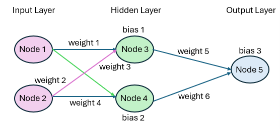
Figure 1 – Neural network

We will also use the terminology and notation from Neural Network Basic Concepts and Neural Network Training and Backward Propagation.

Example Description

Example 1: Here X = (x₁, x₂) and Y = (y), where x₁, x₂, and y only take the values 0 or 1. In particular, the function f(X) = Y that we want the network to compute is f(X) = 0 when x₁ = x₂ and f(X) = 1 otherwise.

There are only 4 possible values for X. These are shown in Figure 2, along with the Y output in each case.

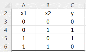
Figure 2 – f(X) = Y

We will use the neural network described in Figure 1. For this simple example, we will use the data shown in Figure 2 as our training set. We will also include all 4 rows in each mini-batch of test data.

Initialization

Rows 10-13 of Figure 3 represent the initial values for the 4 training cases.

We initialize the weights and biases as shown in range A10:I10 of Figure 3 (repeated in rows 11-13 for the other 3 test cases). The values for the two input nodes are shown in range K10:L13 (as copied from Figure 2). The values in range M10:M13 are also copied from Figure 2, although these are not values in the Output node).

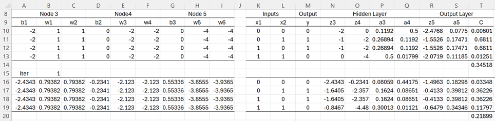
Figure 3 – Initial Steps

The other values in row 10 are calculated as described above using the Excel formulas shown in Figure 4. The values for the other three rows can be obtained by highlighting P10:T13 and pressing Ctrl-D. The cost function for the mini-batch is the average of the 4 costs, as shown in cell T14.

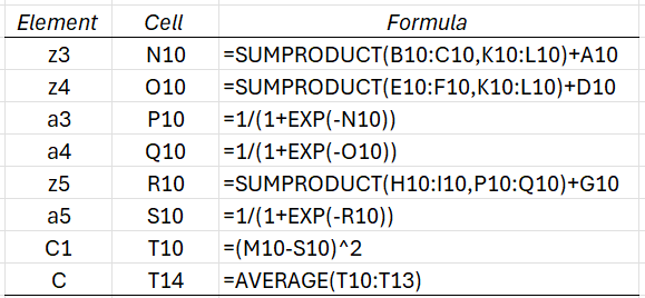
Figure 4 – Key formulas for Figure 3

The output from the neural network is the value of the activation a₅. Activation values close to 0 indicate an output of y = 0, while values close to 1 indicate an output of y = 1. We see from range S10:S13 that at this stage there isn’t much to distinguish between the 4 cases. Clearly, more training is necessary.

Backward propagation

We now use backward propagation to update the biases and weights. This is shown in Figure 5, which displays a continuation of the spreadsheet shown in Figure 3. We also see that the Learning rate has been set to λ = 5.

The values in columns V and W are used to calculate the output layer values in columns Y, Z, and AA. The backward propagation values for the output layer (shown in range Y14:AA14) are then calculated as the average of the individual values.

The values in columns AC – AF are used to calculate the hidden layer values in columns AH – AM. The backward propagation values for the hidden layer (shown in range AH14:AM14) are then calculated as the average of the individual values.

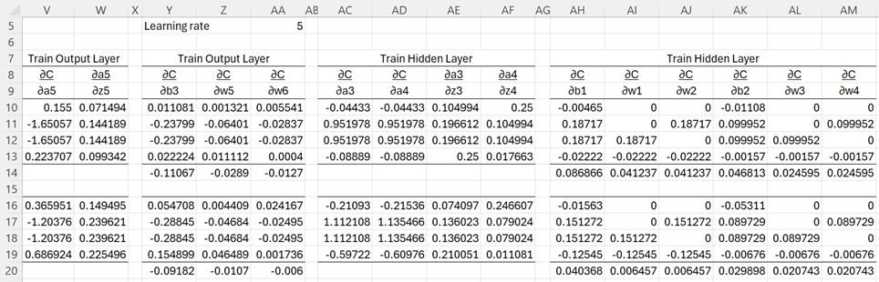
Figure 5 – Backward propagation

The values in row 10 are calculated as described previously using the Excel formulas shown in Figure 6. The values for the other three rows can be obtained by highlighting V10:AM13 and pressing Ctrl-D.

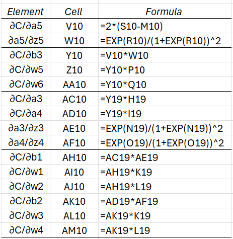
Figure 6 – Key formulas for Figure 5

As stated above, the values in row 14 can be obtained by inserting =AVERAGE(Y10:Y13) in cell Y14, highlighting range Y14:AA14, and pressing Ctrl-R, and then by inserting =AVERAGE(AH10:AH13) in cell AH14, highlighting range AH14:AM14, and pressing Ctrl-R.

Updating the biases and weights

This completes the initial iteration. We now need to update the biases and weights using the backward propagation values calculated above. The updated biases and weights are shown in rows 16-19 of Figure 3. In particular, we place the formula =A10-$M$3*AH14 in cell A16, highlight the range A16:I16, and press Ctrl-R. The values in A17:I17 are just copies of the values for the first training case, and similarly for the other two training cases.

We can now calculate all the other values in rows 16-20 just as we did for rows 10-14. In fact, we can simply copy the formulas in range K10:AM14 into range K16:AM20. We can now copy the formulas in range A16:AM20 into range A22:AM26. We can repeat these steps as many times as we like.

Results

After 20 iterations (i.e. epochs), we obtain the output shown in Figure 7.

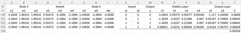
Figure 7 – Results after 20 epochs

We see that the activation levels for the first and last training cases (in column S) are .24658 and .30737, while the middle two training cases are .85167. Since the first two values are less than .5, we can assign them the value of 0. The other two values are greater than .5, and so we assign them the value of 1. This shows that after 20 iterations, we obtain results that match the objective shown in Figure 2.

Note too that the cost function has been reduced to .08354 (cell T134) from .34518 (cell T14 of Figure 3)

If we continue to the 100^th iteration, we obtain activations of .08741, .89509, .89509, .10604, which are even closer to the desired values of 0, 1, 1, 0. The cost function has been reduced to .01022.

Note that different settings for the parameters (initial biases and weights, learning rate, and # of hidden levels) may result in different outcomes.

Examples Workbook

Click here to download the Excel workbook with the examples described on this webpage.

References

Lubick, K. (2022) Training a neural network in a spreadsheet
https://www.youtube.com/watch?v=fjfZZ6S1ad4
https://www.youtube.com/watch?v=1zwnPt73pow

Nielson, M. (2019) Neural networks and deep learning
http://neuralnetworksanddeeplearning.com/