We now show how to design a neural network that can recognize digits 0 – 9 written by hand.
Background
We will assume that the images are written in greyscale. The intensity of the grey can be measured as an integer between 0 and 255, where 0 is black and 255 is white. See Coding a Greyscale Image for a further description.
For our purposes, we will assume that the image is placed over a 28 × 28 grid. Essentially, we are using “pixel art”. Thus, we can code the image as a 28 × 28 array containing integers between 0 and 255. Since 28 × 28 = 784, alternatively, we can code an image as a 1 × 784 row array containing integers between 0 and 255. In this way, we can code k images as a k × 784 row array where each row in the array represents one of the images.
We will use as our training and testing data two data sets provided by the National Institute of Standards and Technology. The first of these MNIST data sets contains 60,000 rows, each row contains the coding for the image of one digit used for training. The second MNIST data set contains 10,000 rows, each row contains the coding for one digit used for testing. These images are scanned hand-written samples from 250 people.
Actually, for our purposes, we will use the first 50,000 rows of the training data set for training and the last 10,000 rows for testing.
Examples of coded images
The first two rows of the MNIST training data are shown in Figure 1 (columns G-EW and FG-ACY are not displayed). Row 2 of this figure displays the 1 × 784 coding for the first image preceded by the fact that this image represents the number 5 (see cell A2).

Figure 1 – MNIST training data
To see the two digits represented by the codes in Figure 1, use the Painting an Image data analysis tool (see Coding an Image Tools) based on inserting B2:ADE3 in the Input Range of the dialog box shown in Figure 4 of Coding an Image Tools, and checking the Greyscale option, making sure that the One Image option is not checked. The output is shown in Figure 2 below.
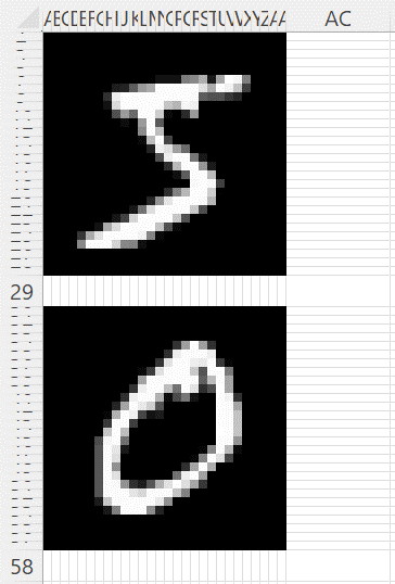
Figure 2 – First two MNIST training images
Since the input contains two rows (recall that the One Image option was not checked), the output in Figure 2 contains two images. These two images are of a 5 and 0, which match the values in cells A2 and A3 of Figure 1.
Neural network description
We now train a neural network to recognize images of digits 0 – 9 using the first 50,000 rows of the MNIST training data. Our network will contain 784 input nodes, 10 hidden nodes, and 10 output nodes. See Neural Network Basic Concepts for details.
Training data
Before we start, we reformat the MNIST data so that the y values appear after the X data and the greyscale codes take values between 0 and 1 (instead of 0-255). This is done by dividing each of the 0-255 codes by 255. The first two rows of this revised data are shown in Figure 3.

Figure 3 – MNIST training data reformatted
The 50,000 rows of revised training data fill in the range B2:ADF50001.
Initializing the neural network
We use the Training a Neural Network data analysis tool to train our neural network (as described in Neural Network Analysis Tools). We start by filling in this tool’s dialog box as shown in Figure 4.
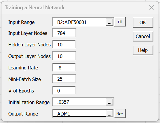
Figure 4 – Training a Neural Network dialog box
As you can see from the figure, we set the # of epochs to zero and the learning rate to .8. We also insert .0357 in the Initialization Range field, which means that all the biases and weights are initially set to random values from the normal distribution with mean zero and standard deviation .0357.
Note that we could have simply left the Initialization Range field blank. In this case, all the biases and weights would have been set to the default values, namely random values from the normal distribution with mean zero and standard deviation 1/√784 = .035714.
Training the network
After pressing the OK button on the dialog box, we obtain the biases and weights shown in range ADN7:ADN7968 (most of which is not displayed) of Figure 5.
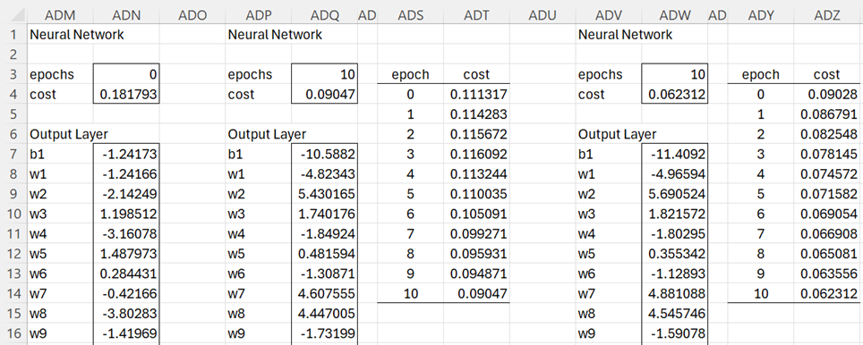
Figure 5 – Training using MNIST data
We now continue the training for 10 epochs by again pressing Ctrl-m, selecting Training a Neural Network from the Corr tab, and entering the same values in the dialog box as those that appear in Figure 4 except that this time we insert 10 in the # of Epochs, ADN7 in the Initialization Range and ADP1 in the Output Range.
The results are shown in columns ADP – ADT of Figure 5. We see that the cost function starts in the right direction (decreasing from .181793 in cell ADN4 to .111317 in cell ADP4), but then starts increasing (from .111317 to .116092) before it starts decreasing again down to .09047 (slowing down in the last epoch from .090471 to .090470).
We now decrease the learning rate to address this somewhat erratic behavior of the cost function and run another 10 epochs using a learning rate of .5 starting using the biases and weights in ADQ7:ADQ7968.
Testing the accuracy of the network
Having obtained a cost function of .062312 (cell ADW4), we decide to test the accuracy of the neural network. We do this by pressing Ctrl-m, selecting the Training a Neural Network option from the Corr tab, and filling in the dialog box that appears as shown in Figure 6.
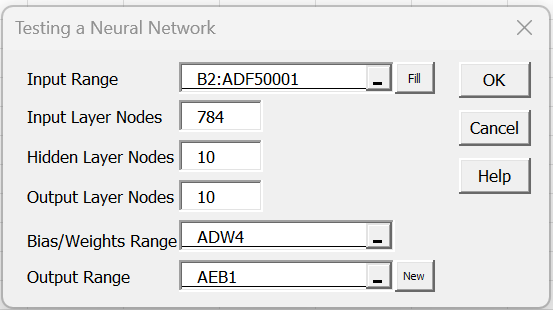
Figure 6 – Testing a Neural Network dialog box
After pressing the OK button, we obtain the results shown in Figure 7.
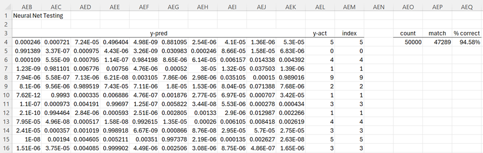
Figure 7 – Testing results (first 11 rows displayed)
The figure only shows the first 11 of 50,000 rows of test results. The values in column AEL come from column ADF (in Figure 3) of our original data. Column AEM contains the digit predicted by the neural network. For row 4 the largest activation occurs in column AEG, which is the 6th column in the output.
Since the first column represents the digit 0, the second column represents the digit 1, etc., the 6th column represents the digit 5, as shown in cell AEM4. Thus the network correctly predicts the first training image. In fact, we see from comparing columns AEL and AEM, that the network correctly predicts the first 11 training images.
Overall, of the 50,000 training images, the network correctly predicts 47,289 images (cell AEP4) for 94.58% accuracy.
Overfitting
While achieving 94.58% accuracy seems pretty impressive, at least to me, after only 20 epochs, a word of caution is needed. After all, we are testing the accuracy of the network based on the same 50,000 images that we have been training the network on. Perhaps the network gives reasonable results for these images, but how will it do on new images that it hasn’t seen before?
In fact, there is always the danger that the network performs extremely well on the training data, but not so well on new data. This is a problem of overfitting.
Testing using new data
To overcome this deficiency, we repeat the testing using the last 10,000 images in the training dataset that the network has never seen before. We do this using the Testing a Neural Network data analysis tool inserting B50002:ADF60001 in the Input Range of the dialog box in Figure 6 to obtain the results shown in Figure 8 (only the first 11 rows are displayed).
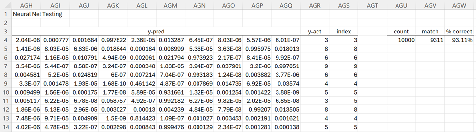
Figure 8 – Testing on 10,000 new images
We see that the accuracy using the test data is 93.11%. Although less than the 94.58% using the training data, this level of accuracy is pretty good.
Investigating an image not predicted correctly
We see from Figure 8 that the network predicts that the 8th testing image is a 5 while the image is supposed to represent a 3. Using the Painting an Image data analysis tool, as explained in Coding an Image Tools, we see that the actual image is as shown in Figure 9.
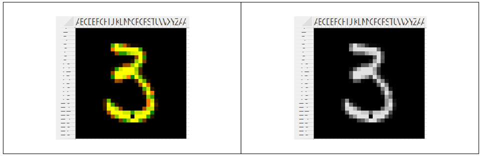
Figure 9 – Actual image of a 3
We produced the image on the left side of Figure 9 by inserting B50009:ADE5009 in the Input Range of the dialog box for the Painting an Image data analysis tool, checking the Greyscale option, and unchecking the One Image option (since the data in the input range is in row format).
Surprisingly, the image is displayed in color. This is because B50009:ADE5009 doesn’t contain the original greyscale color codes (0-255). Instead, it contains these codes divided by 255. We would have seen the greyscale image shown on the right side of Figure 9 if we had used the original MNIST data. To obtain the greyscale version, we could use the Convert to Greyscale data analysis tool.
In any case, the human eye sees a 3, but the neural network isn’t able to differentiate this from a 5. Note that the first item in the test data is also a 3 (cell AGR4 in Figure 8), but the network was able to correctly differentiate this 3 from a 5.
Continued training and testing
We continue to train the network using 50,000 images in the training dataset for another 35 epochs varying the learning rate between .18 and .40 in runs of size 5 epochs, arriving at the results shown in Figure 9.
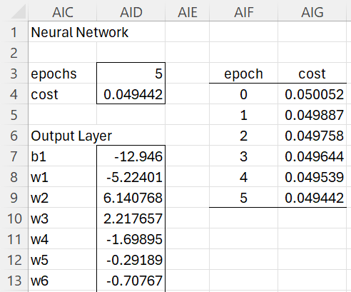
Figure 9 – Training results after 45 epochs
We have managed to reduce the cost from .062312 in Figure 5 to .049442 in Figure 9. We have also increased the accuracy on the 50,000 training images from 94.58% to 95.08% and on the 10,000 testing images from 93.11% to 93.21%, as shown in Figure 10.
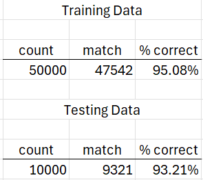
Figure 10 – Revised test results
Conclusions
The additional training seems to improve the accuracy when the training data is used more than when the testing data is used. In fact, if we were to add another 60 epochs of training, we would decrease the cost function from .49442 to .45902 and increase the accuracy for the training data from 95.08% to 95.36. However, the accuracy using the testing data would actually decrease from 93.21% to 93.16%.
Perhaps we are reaching the limits of the training of the neural network and starting to overfit the network to the training data. To improve the accuracy of the network further, we might need to use a different approach. For example, increasing the number of hidden nodes might be useful. Using all the 60,000 training images for training and using the separate 10,000 images in the testing database might also help. Different cost functions or activation functions might also be useful.
Examples Workbook
Click here to download the Excel workbook (size: 238 megabytes) with the examples described on this webpage.
Links
References
Lubick, K. (2022) Training a neural network in a spreadsheet
https://www.youtube.com/watch?v=fjfZZ6S1ad4
https://www.youtube.com/watch?v=1zwnPt73pow
Nielson, M. (2019) Neural networks and deep learning
http://neuralnetworksanddeeplearning.com/