We now show how to use Real Statistics’ neural network data analysis tools to build a network that solves a problem a little more complicated than the XOR gate described in Simple Neural Network.
Example
Example 1: Construct a neural network that performs addition on the numbers 0, 1, and 2, as shown in Figure 1.
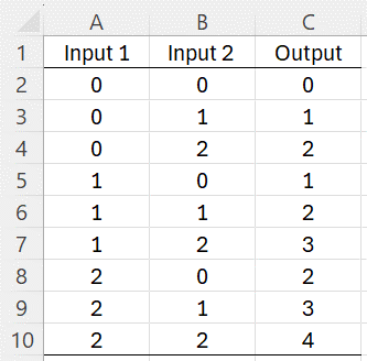
Figure 1 – Addition Function
This time we are dealing with a function with two inputs X = (x1, x2) and five outputs Y = (y1, y2, y3, y4, y5). We are asking the neural network to compute f(X) = Y where x1 and x2 take the values 0, 1, or 2 and y1, y2, y3, y4, and y5 all take the values 0 or 1. E.g. row 7 in Figure 1 actually calculates f(1, 2) = (0, 0, 0, 1, 0). The output is a vector with 4 zeros and one 1. The position of the 1 determines the output in column C of Figure 13 where the first position (i.e. y1) corresponds to 0, the second position (i.e. y2) corresponds to 1, etc.
Once again, we will use the Real Statistics Training a Neural Network data analysis tool using the data in Figure 1 as the training set. To keep things simple the Real Statistics data analysis tool already knows that y = 3 is really an abbreviation for Y = (0, 0, 0, 1, 0), and so we can use the format provided in Figure 1.
Initialization
As explained in Neural Network Analysis Tools, we press Ctrl-m and select the Training a Neural Network option from the Corr tab. Next, we fill in the dialog box that appears as shown in Figure 2.
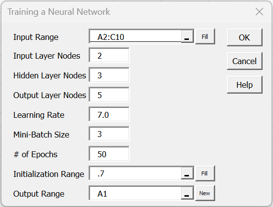
Figure 2 – Training Dialog Box
This time, we use a network with 2 input nodes, 3 hidden nodes, and 5 output nodes, and set the Learning Rate to 7.0. Since we don’t have much training data, we could use all nine rows of data from Figure 2 as a mini-batch by setting the Mini-Batch Size field to 9. Instead, we will divide the training into 3 mini-batches each of size 3. We specify 50 epochs (which results in 50 × 3 = 150 times that we perform backward propagation.
This time, instead of setting the Initialization Range to 0 or filling in a range of biases and weights, we supply the number .7. This instructs the neural network to assign to each bias and weight a random value from the normal distribution with mean zero and standard deviation .7.
If we had used -.7 instead, then the neural network would have assigned a random value between -.7 and +.7 to every bias and weight in the network.
Thus, if a positive value r is used then the biases and weights are assigned random values from a normal distribution with mean 0 and standard deviation r, while if a negative value –r is used, then the biases and weights are assigned random values from the uniform distribution between –r and r. Using the value 0 assigns the fixed values of b = -1 and w = +1 to all the biases and weights.
Leaving the Initialization Range empty is equivalent to assigning the value 1/√n1 (where n1 = the number of input nodes).
Output
After clicking on the OK button, the results are as shown on the left side of Figure 3 (with rows 13 to 48 omitted from the display). We see that the cost function has decreased from .881843 to .430969. For the most part, the cost function continuously decreased, although occasionally it increased (e.g. from epoch 1 to 2, and from epoch 4 to 5), which is often a sign that the Learning Rate is set too high. It can also be a way to shift the algorithm from a dead-end to a more promising path.
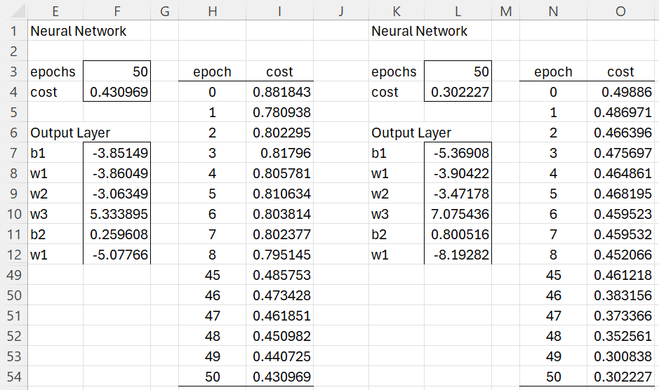
Figure 3 – Training (first 100 epochs)
Testing
We can test the accuracy of the neural network by using the Testing a Neural Network data analysis tool, as described in Neural Network Analysis Tools. Here we press Ctrl-m, select the Testing a Neural Network option from the Corr tab, and then fill in the dialog box that appears as shown in Figure 4.
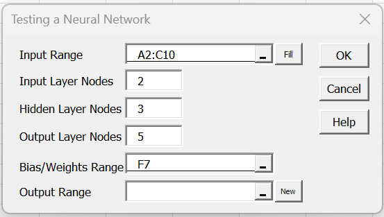
Figure 4 – Testing dialog box
Here the Bias/Weights Range of F7 refers to the first cell of range F7:F17 of Figure 3 containing the current biases and weights.
Since the total amount of potential data is limited to the same nine cases used for training, we need to reuse these cases for testing.
After clicking on the OK button, the output shown in Figure 5 appears.
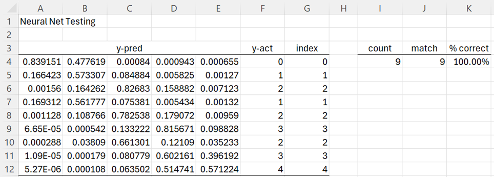
Figure 5 – Revised testing results
This time, the network matches all nine of the test cases. The y = 2 prediction for 0 + 2 in row 6 is quite solid since .82683 (cell C6) is clearly much larger than any of the other choices in row 6. The y = 4 prediction for 2 + 2 = 4 in row 12 is far less solid since .571224 (cell E12) is only a little bigger than .514741 (cell D12).
More Epochs
We now add another 50 epochs (with Learning Rate = 3.0) as shown on the right side of Figure 3. We now arrive at a clearer difference between the values in row 12, namely, .218105 vs. .820463, as shown in Figure 6.
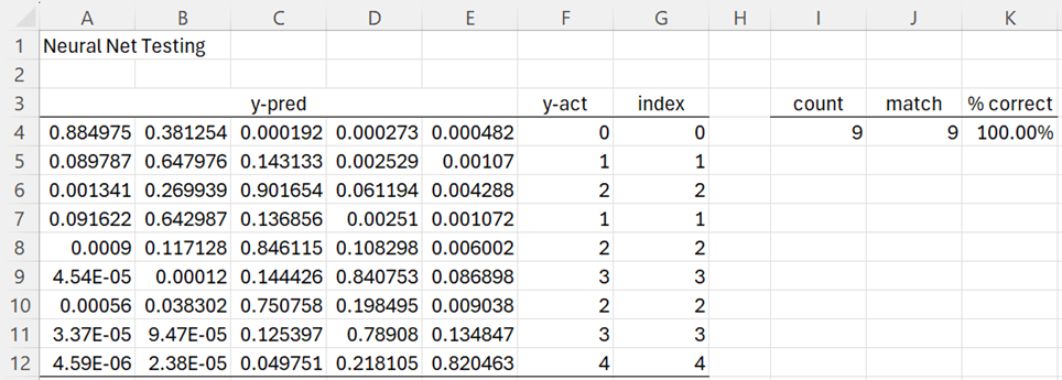
Figure 6 – Improved testing results
Observation
Note that there is a certain amount of trial and error before you can obtain acceptable results. Often, you need to tweak some of the parameters (e.g. the number of hidden layer nodes, the learning rate, the initial biases and weights, and the number of epochs).
Examples Workbook
Click here to download the Excel workbook with the examples described on this webpage.
Links
References
Lubick, K. (2022) Training a neural network in a spreadsheet
https://www.youtube.com/watch?v=fjfZZ6S1ad4
https://www.youtube.com/watch?v=1zwnPt73pow
Nielson, M. (2019) Neural networks and deep learning
http://neuralnetworksanddeeplearning.com/