Multivariate Normal Distribution and GHK Algorithm

On this webpage we describe the GHK (Geweke, Hajivassiliou and Keane) sampling algorithm and how to use it to estimate the cdf of the multivariate normal distribution (see Multivariate Normal Functions).

GHK Algorithm

Let N(μ, Σ) be a multivariate normal distribution where μ is the k × 1 mean-vector and Σ is the k × k covariance matrix. Also, let A and B be k × 1 vectors where A < B (i.e. a_i < b_i for all i). We can assume that μ is the zero vector.

Our goal is to create a sequence of k × 1 vectors X₁, …, X_r, such that A < X_j < B for all j. We can then use this sequence to estimate P(A < X < B) via the formula

where

and the q_im are defined recursively using the Cholesky decomposition of Σ = CC^T. Note that c_ij = 0 if j > i. For i = 1, we define

and for i = 2, 3, …, k (and m = 1, …, r), define q_im recursively as follows:

where Φ(x) = the standard normal distribution function at x, which can be calculated in Excel by =NORM.S.DIST(x,TRUE), and

with ε_hm drawn randomly from a truncated normal distribution with bounds

Example

Example 1: Approximate P(A < X < B) for the bivariate normal distribution defined in Example 1 of Multivariate Normality Functions on the bounds A = (10, 15) and B = (20, 30) using the GHK algorithm with 10 samples.

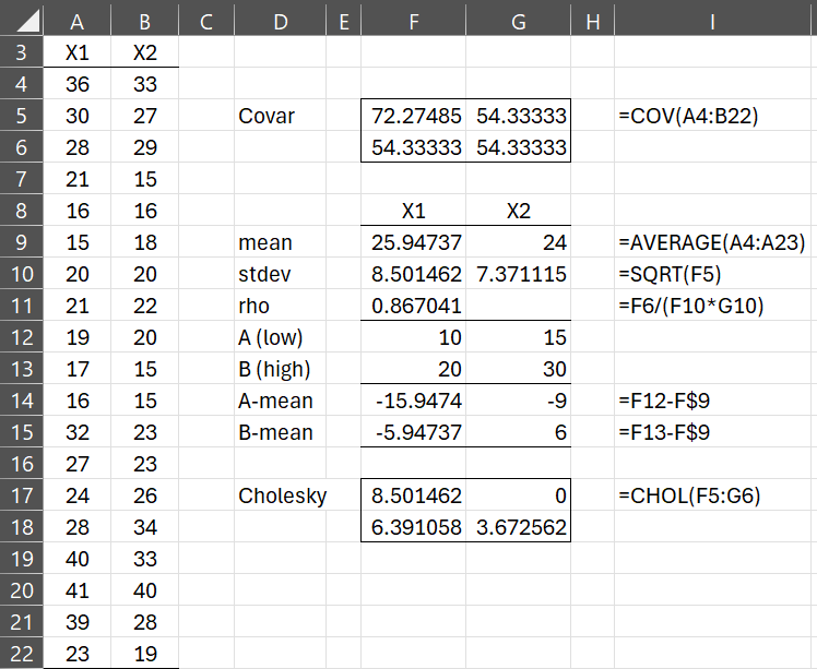
Figure 1 shows the data and associated parameters for this bivariate normal distribution.

Figure 1 – Example bivariate normal distribution

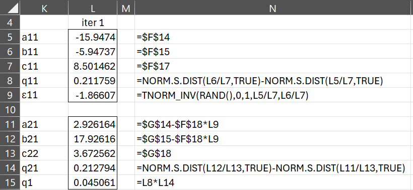
Figure 2 describes how to obtain the first sample used in the GHK algorithm.

Figure 2 – Sample 1 of GHK algorithm

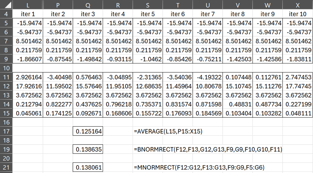
We obtain the other nine samples in exactly the same way, with the results shown in Figure 3.

Figure 3 – 10 Samples using the GHK algorithm

The estimated probability is the average of the 10 q_j values in row 15, namely .125164 (cell S17). Note that if we use the Real Statistics MNORMRECT worksheet function with 200 samples (instead of 10), we obtain a better estimate of .138635 (cell S21). We can get a fairly good estimate with a relatively small sample.

We define this function momentarily. We can also use the BNORMRECT, defined in Multivariate Normal Functions, to obtain the result shown in cell S19. Of course, the advantage of the MNORMRECT function is that it applies to any multivariate normal distribution, not just bivariate normal distributions.

Multivariate Normal CDF

We can use the GHK algorithm to calculate the cumulative distribution function (cdf) of a multivariate normal distribution. To calculate the cdf F(X) for random vector X, we set the upper bound B in the GHK algorithm to X and the lower bound to A = a vector all of whose values are -∞. We can accomplish this by using a sufficiently large negative value such as -100 (or even -10) instead of -∞. Alternatively, we can replace Φ(a_im/c_ii) by zero in the GHK algorithm.

Using the GHK algorithm in this way with 200 samples, we estimate the cdf of the multivariate normal distribution in Example 1 at X = (10, 15) to be F(X) = .02757, as shown in Figure 4.

Figure 4 – CDF using the GHK algorithm

Actually, we use the MNORMDIST worksheet function, as described below, to obtain these results. We obtain similar results using the BNORMDIST worksheet function.

Worksheet Functions

Real Statistics Functions: The Real Statistics Resource Pack provides the following functions in support of multivariate normal distributions.

MNORMDIST(R0, Rm, Rc, cum, iter) = the cdf of the multivariate normal distribution at R0 if cum = TRUE and the pdf if cum = FALSE.

MNORMRECT(Rlo, Rhi, Rm, Rc, iter) = P(A < X < B) for the multivariate normal distribution where A and B are the column vectors corresponding to Rlo and Rhi.

Here, R0, Rm, Rlo, and Rhi are k × 1 arrays or cell ranges with all the elements in Rlo less than or equal to the corresponding element in Rhi. Rm represents the mean vector and Rc is the k × k covariance matrix. iter = the number of samples used in the GHK algorithm (default 200).

Examples Workbook

Click here to download the Excel workbook with the examples described on this webpage.

References

Greene, W. (2012) Econometric analysis, 7^th ed. Prentice Hall
https://bayanbox.ir/view/7862953811569997962/econometric-Analysis-Greene.pdf

Wikipedia (2024) GHK algorithm
https://en.wikipedia.org/wiki/GHK_algorithm

Shum, M. (2008) GHK description
https://www.its.caltech.edu/~mshum/gradio/ghk_desc.pdf