Two-way MANOVA

Two-way MANOVA can be considered to be an extension of one-way MANOVA to support two factors and their interaction or as an extension to two-way ANOVA to support multiple dependent variables.

Univariate case

Two-way ANOVA investigates the effects of two categorical variables on a continuous outcome (the dependent variable). In two-way ANOVA, we have r random variables (the levels) for Factor A (the row factor) and c random variables for Factor B (the column factor). For each interaction between the factor levels, we have a sample with m elements (we restrict ourselves to the balanced model here). We can represent the sample for the i^th level from Factor A and the j^th level from Factor B by X_ij = {x_ij1, …, x_ijm}.

Our objective is to test three types of null hypotheses:

H₀: μ_1. = μ_2. = … = μ_r.  (Factor A)

H₀: μ_.1 = μ_.2 = … = μ_.c  (Factor B)

H₀: δ_ij= 0  for all i, j (Interaction between A and B, where the δ_ij  are the interaction effects

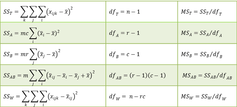
We define the following where n = mrc.

The test statistics F are defined as follows:

For each of the three null hypotheses, we reject the null hypothesis if F > F_crit.

Multivariate case

As for one factor MANOVA, two-factor MANOVA is similar to two-factor ANOVA except that in place of simple variables (for each factor) we have random vectors and in place of sample data {x_ij1, …, x_ijm} for the i^th level in Factor A and the j^th level in Factor B, we have sample data {X_ij1, …, X_ijm}  where each X_ijk is a p × 1 column vector of data elements of the form x_ijkh. Here, there are p dependent variables.

The additive model takes the form:

This is exactly as for a two-factor ANOVA model except that x_ijk is replaced by X_ijk and the other terms are column vectors instead of scalars. With this change, the null hypotheses are as for ANOVA. In place of the ANOVA normality assumption, assume multivariate normality, namely

The df terms are as for ANOVA, as defined above, and the SS terms are defined in terms of the following p × p cross-product matrices.

Recall from MANOVA Basic Concepts, that each of these SS matrices takes the form

where for SS_A

and similarly for the other SS matrices.

Wilk’s Lambda

Each of the three null hypotheses is tested using the appropriate Wilk’s Lambda.

If the Factor H null hypothesis is true (for H = A, B or AB) then

As for one factor MANOVA, a more accurate test is based on the F test, described as follows:

where

If either the numerator or denominator of b equals 0 or results in a negative value inside the square root, then b takes the value of 1.

Hotelling-Lawley Trace

Each of the three null hypotheses is tested using the appropriate Hotelling-Lawley Trace test.

where

Pillai-Bartlett Trace

Each of the three null hypotheses is tested using the appropriate Pillai-Bartlett Trace test.

where Roy’s Largest Root

Each of the three null hypotheses is tested using the appropriate Roy’s Largest Root test.

where

and s, t, u are as for the Pillai-Bartlett Trace test.

References

Ender, P. (2007) Multivariate Statistical Analysis
This document is no longer available on the Internet

Tsay, R.S. (2016) Applied Multivariate Analysis

Penn State (2023) Two-way MANOVA additive model and assumptions
https://online.stat.psu.edu/stat505/lesson/8/8.10