One Sample Hotelling’s T-square

Univariate case

As described in One Sample t-Test, the t-test can be used to test the null hypothesis that the population mean of a random variable x has a certain value, i.e. H₀: μ = μ₀. The test statistic is given by

The applicable univariate test of the null hypothesis is based on the fact that t ~ T(n–1) provided the following assumptions are met:

• The population of x has a unique mean: i.e. there are no distinct sub-populations with different means
• The population of x has a normal distribution
• The data consists of a random sample with each element in the sample taken independently

Regarding the normality assumption, if n is sufficiently large, the Central Limit Theorem holds, and we can proceed as if the population were normal. It turns out that the t-test is pretty robust to violations of the normality assumption provided the population is relatively symmetric about the mean.

The null hypothesis is rejected if |t| > t_crit. Also, by Property 1 of F Distribution, an equivalent test can be made using the test statistic t² and noting that t² ~ F(1, n – 1).

Now, t² can be expressed as follows:

where x̄ is the sample mean and s is the sample standard deviation.

Multivariate case

Experiment-wise error

We now look at a multivariate version of the t-test, which decides whether the population mean of the k × 1 random vector X has a certain value. Here, the null hypothesis is H₀: μ = μ⁰ where μ and μ⁰ are vectors.

Since the null hypothesis is true when μ_i = μ_i⁰ for all i, 1 ≤ i ≤ k, one way to carry out this test is to perform k separate univariate t-tests (or the equivalent F tests). The null hypothesis is then rejected if any one of these k univariate tests rejects its null hypothesis.

As we observed in Experiment-wise Error Rate, this approach introduces experiment-wise error, namely, if we use a given value of α for all k tests, then the probability of the multivariate null hypothesis being rejected is much higher than α. For this reason, we typically use a correction factor, usually, the Dunn/Sidák or Bonferroni correction factor, as described in Planned Comparisons. Thus, we use a significance level of 1 –(1–α)^1/k or α/k instead of α for each of the k univariate tests.

This approach is perfectly reasonable when the random variables x_i in X are independent. But when they are not independent then the Dunn/Sidák or Bonferroni correction factors over-correct and the resulting experiment-wise value for α is lower than it needs to be, which results in a test with lower statistical power.

Since it is common to create experiments in which the random variables x_i in X are not independent, it is better to use a different approach. In particular, we will use the multivariate test based on Hotelling’s T-square test statistic.

T-square statistic

Definition 1: Hotelling’s T-square test statistic is

where S is the covariance matrix of the sample for X, X̄ is the mean of the sample, and the sample has n elements.

Note the similarity between the expression for T² and the expression for t² given above.

Property 1:

Corollary 1: By the multivariate version of the Central Limit Theorem, for n sufficiently large, T² ~ χ² (k).

For small n, Property 1 doesn’t yield results that are sufficiently accurate. A better estimate is achieved using the following property.

Property 2: Under the null hypothesis

If F > F_crit then we reject the null hypothesis.

Example

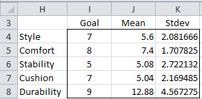
Example 1: A shoe company evaluates new shoe models based on five criteria: style, comfort, stability cushioning, and durability. Each of the first four criteria is evaluated on a scale of 1 to 20 and the durability criterion is evaluated on a scale of 1 to 10. Column I of Figure 1 shows the goals for each criterion expected from new products.

Figure 1 – Product goals by criteria

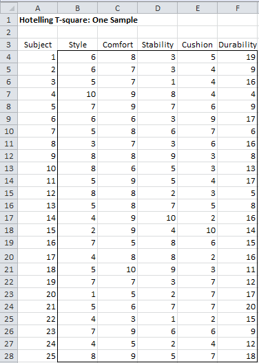
Based on the evaluations of 25 people about the company’s latest prototype (Model 1) shown in Figure 2, determine whether the shoe is ready for release to the market.

Figure 2 – Sample data for Example 1

The sample mean and standard deviation for each criterion are shown in columns J and K of Figure 1. The sample covariance and correlation matrices are then calculated using the Real Statistics array formulas COV(B4:F28) and CORR(B4:F28), as shown in Figure 3.

Figure 3 – Covariance and Correlation Matrices

Results

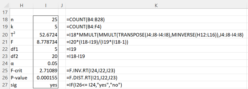
Using Definition 1 and the data in Figures 1, 2, and 3, we can calculate T² as shown in cell I20 of Figure 4. Since the formula used to calculate T² is an array formula (even though it yields a scalar numeric result), it is important to press Ctrl-Shft-Enter after entering the formula in cell I20 (unless using Excel 365 where this is not necessary).

Figure 4 – Hotelling T² test for a single sample

As we will see shortly, you can also obtain T² by using the formula

=HotellingT2(B4:F28,I4:I8)

which employs the Real Statistics function HotellingT2 found in the Real Statistics Resource Pack. Note that this formula is not an array formula and so it is sufficient to press Enter after entering the formula. 

We can determine whether there is a significant difference between the sample means in the five categories and the goals (i.e. population means) by using Property 2. As can be seen from Figure 4, since p-value < .05 (or F > F_crit), we reject the null hypothesis and conclude there is a significant difference between the mean scores in the sample and the stated goals.

Confidence intervals

Example 2: For the prototype shoe in Example 1, determine which criteria meet the goals and which do not.

We can test each criterion using a One Sample t-Test. The results of this analysis are shown in Figure 5.

Figure 5 – T-test for each criterion

From Figure 5, we can conclude that Style and Cushioning are significantly below the goals. Durability is significantly higher than the goals and Comfort and Stability are within the goals.

Figure 5 includes the 95% confidence intervals for each criterion. In the univariate case, the 1–α confidence interval for the population mean μ is based on

which nets out to the interior of the interval

The problem with this analysis is that we haven’t taken experiment-wise error into account. In fact, the combined (worst-case) error rate is 1-(1-.05)⁵ = .226 instead of .05.

If the random variables representing the 5 criteria were independent, then we could compensate for this by applying either the Dunn/Sidák or Bonferroni correction factor. As we can see from the correlation matrix in Figure 2, the variables are clearly not independent since some of the values off of the main diagonal are far from zero.

Simultaneous intervals

In order to control for experiment-wise error, we instead calculate the 95% confidence ellipse (using Property 2) which takes all 5 criteria into account simultaneously. In particular, we use the following modified version of the observation which follows Property 3 of Multivariate Normal Distribution Basic Concepts, noting that based on Definition 1 and Definition 3 of Multivariate Normal Distribution Basic Concepts, T² is approximately n times the Mahalanobis distance between X-bar and μ⁰.

Using Property 2, we have a 1 – α confidence hyper-ellipse for the population mean vector μ which is given by

Thus, we are looking for values of μ which fall within the hyper-ellipse given by the equation

From the 1–α confidence hyper-ellipse, we can also calculate simultaneous confidence intervals for any linear combination of the means of the individual random variables. For example, for the linear combination

the 1 – α simultaneous confidence interval is given by the expression

where the sample covariance matrix is S = [s_ij].

For the case where c = μ_i the 1–α simultaneous confidence interval is given by the expression

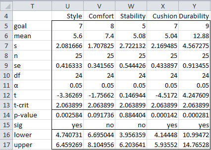
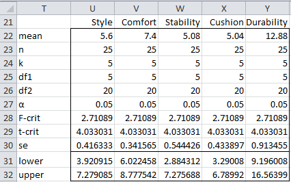
where s_i is s_ii = the standard deviation of the x_i. Since the 1–α confidence intervals for all linear combinations are a manifestation of the 1–α confidence hyper-ellipse, it follows that the following are simultaneously the 95% confidence intervals for all 5 criteria:

Figure 6 – Simultaneous 95% confidence intervals

Most of the cells in Figure 6 already appear in Figure 4. The value of t-crit (e.g. cell U29) is derived from F-crit using the formula =SQRT(U24*(U23-1)/(U23-U24)*U28). The value of the lower bound of the 95% confidence interval for Style is calculated by the formula =U22-U29*U30, and similarly for the upper and lower bounds of the other criteria.

We summarize the conclusions from this analysis in Figure 7.

Figure 7 – Comparison of simultaneous intervals with goals

From Figure 7, we conclude that Cushioning is significantly below the goals, Durability is significantly higher than the goals and the other criteria are within the goals set by the company.

Bonferroni intervals

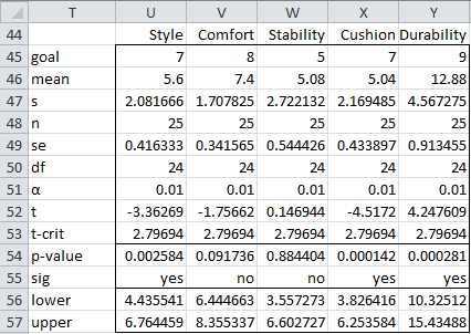
The simultaneous confidence intervals handle all linear combinations of the means, but since we are only interested in the individual means, the stated confidence intervals may be too wide. In this case, we might be better off using the Dunn/Sidák or Bonferroni correction factor. The calculations for the Bonferroni correction factor are similar to those in Figure 5, except that we use the experiment-wise value of alpha = α/k = .05/5 = .01. The results are shown in Figure 8.

Figure 8 – Bonferroni confidence intervals

The confidence intervals in Figure 8 are narrower than those in Figure 7 and the overall conclusions are a little different, as shown in Figure 9.

Figure 9 – Comparison of Bonferroni intervals with goals

Although we will generally use the hyper-ellipse based on F as described above, for large samples, based on Corollary 1, we could also use the following 1–α confidence hyper-ellipse for any linear combination c of the means:

Where c = μ_i, this nets out to

Effect Size and Power

Click here for two measures of effect size for the one-sample Hotelling’s T-square test as well as how to calculate the power of this test.

References

Penn State University (2013) Hotelling’s T-square. STAT 505: Applied multivariate statistical analysis (course notes)
https://online.stat.psu.edu/stat505/lesson/7/7.1/7.1.3

Rencher, A.C. (2002) Methods of multivariate analysis (2nd Ed). Wiley-Interscience, New York.
https://www.ipen.br/biblioteca/slr/cel/0241

Johnson, R. A. and Wichern, D. W. (2007) Applied multivariate statistical analysis. 6th Ed. Pearson.
https://www.webpages.uidaho.edu/~stevel/519/Applied%20Multivariate%20Statistical%20Analysis%20by%20Johnson%20and%20Wichern.pdf