Jenks Natural Breaks

Jenks Natural Breaks optimization addresses the problem of how to split a range of numbers into contiguous classes so as to minimize the squared deviation within each class.

Example

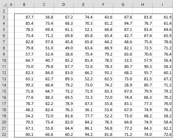
Example 1: Define 4 classes for the data in Figure 1 which achieves this objective.

Figure 1 – Data for Example 1

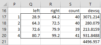
Suppose, for example, that we simply divide the 160 elements in Figure 1 into four intervals each containing 40 elements, as shown in Figure 2.

Figure 2 – Equally spaced intervals

Here, for example, cell Q18 contains the formula =SMALL($B$3:$I$22,40*(P18-1)+1), cell R18 contains the formula =SMALL($B$3:$I$22,40*P18) and cell S18 contains the formula

=COUNTIFS($B$3:$I$22,”>=”&Q18,$B$3:$I$22,”<=”&R18)

Note that cell R19 should contain the 120^th smallest element in Figure 1, which is 80.7, but since 80.7 is also the 121^st smallest element, this would split 80.7 between interval 3 and interval 4. This is why we are forced to make interval 3 slightly smaller and interval 4 slightly bigger.

The squared deviation of each of the four intervals is found in range T17:T20, with the sum in cell T21. Note that cell T17 contains the array formula

=DEVSQ(IF($B$3:$I$22>=Q18,IF($B$3:$I$22<=R18,B4:I23,””),””))

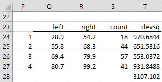
What we don’t know is whether this choice of four intervals is the partition of the full range that results in the smallest sum in cell T21. As we will see shortly, the optimum solution, using Jenks Natural Breaks optimization, is shown in Figure 3. As you can see, this is a better solution than the one shown in Figure 2 (since 3107.102 < 4496.957).

Figure 3 – Optimal partition

Small Example

Example 2: Find the optimal partition of the values 5, 8, 9, 12, and 15 into 3 classes.

Since this is a simpler problem than the one in Example 1, we are able to evaluate all six possible solutions, as shown in Figure 4.

Figure 4 – Jenks Natural Breaks

In the first possible solution, shown in range B3:D7, the three classes are 5, 8, and 9-15. The squared deviation for the third category (cell D6), for example, is calculated by the formula =DEVSQ(D3:D5), with a total for all three classes of 18, using the formula =SUM(B6:D6).

We see from Figure 4 that the optimal partition is the second one, with classes 5, 8-9, and 12-15 since the total squared deviation of 5 is less than that of the other partitions.

The value of 5 is repeated in cell AA4 in order to calculate the goodness of variance fit (GVF), which is calculated as

GVF =

where d* is the minimum total squared deviation, as described above, and d is the squared deviation of the data set, which for Example 2 is 58.8 (cell AA3) as calculated by the formula =DEVSQ(F3:H5). GVF takes a value between 0 and 1. The closer to 1 the better the fit.

Iterative Approach

In Example 2, we were able to go through each possible partition and calculate its squared deviation. While in Example 1, this is too time-consuming to do manually, we can use the Real Statistics Jenks Natural Breaks data analysis tool, as described below, to do the calculations for us, for other problems the number of possible partitions is even too time-consuming for the computer to do.

For example, there are 8,301,429,675 ways to partition 254 data elements into 6 classes. This number gets even larger the more data elements there are and the more classes we want to use.  In such cases, we will need to use an iterative approach. In particular, we select a partition at random and see which class has the largest squared deviation and which class has the least squared deviation.

If, for example, we used 6 classes and class 3 had the largest squared deviation and class 5 had the smallest squared deviation, then we would move the last element in class 3 into class 4 (in the direction of class 5). If instead, class 3 had the largest squared deviation and class 1 had the smallest squared deviation, then we would move the first element in class 3 into class 2.

We repeat this process again and again, continuing until the squared deviations of none of the classes changed or until a maximum number of iterations had been reached, at which point we would select the partition with the lowest total squared deviations. In order to avoid a local minimum, from time to time we could make a random perturbation.

Data Analysis Tool

Real Statistics Data Analysis Tool: The Real Statistics Resource Pack provides the Jenks Natural Breaks data analysis tool to perform the optimization automatically.

To perform the analysis for Example 1, press Ctrl-m and select Jenks Natural Breaks from the Multivar tab. If you are using the original user interface, then instead choose the Multivariate Analyses option from the main menu and then select Jenks Natural Breaks from the dialog box that appears.

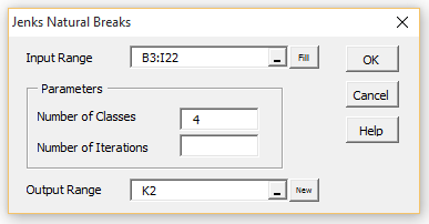
In either case, the Jenks Natural Breaks dialog box will now appear. Fill in the various fields as shown in Figure 5 and press the OK button. If you leave the Number of Iterations field blank then the algorithm will evaluate all possible partitions.

Figure 5 – Jenks Natural Breaks dialog box

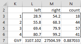
The result is shown in Figure 6.

Figure 6 – Jenks Natural Breaks data analysis

Here 3107.102 (cell L7) represents the total squared deviation for the partition found using the Jenks Natural Breaks algorithm, 27504.59 (cell M7) is the squared deviation of the input data, as calculated by =DEVSQ(B3:I22), and 88.7% is the GVF (cell N7), as calculated by the formula =1-L7/M7.

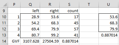
As described earlier, for large data sets or a large number of classes (especially 6 or 7 or greater), you should usually use an iterative approach by filling in the Number of Iterations field with a number such as 10000 or 250000 to specify the maximum number of iterations. Figure 7 contains the output for Example 1 with 100,000 iterations.

Figure 7 – Iterated version of Jenks Natural Breaks

Note that the GVF of .887014 is only slightly lower than the optimal solution shown in Figure 6. Note too that if you run the algorithm again with 100,000 iterations, you may get a slightly different solution.

Worksheet Functions

Real Statistics Functions: The Real Statistics Resource Pack provides the following functions.

JENKS(R1,, lab, iter) – performs Jenks Natural Breaks optimization on the data in range R1 for k classes and outputs a k+1 × 3 range, whose first k rows contain the left and right endpoints of each of the classes followed by the number of elements in the class. The last row contains the total squared deviation of the k classes, followed by the squared deviation for the data in R1 and GVF.

Here k+1 = the number of rows in the highlighted output range. If iter is included then the algorithm uses iter iterations, otherwise, all possible partitions are tested. If lab = TRUE (default = FALSE) then an extra column of labels is included.

The range K3:N7 of Figure 7 contains the output of the array formula =JENKS(B3:I22,,TRUE). The range P10:S14 of Figure 8 contains the output of the array formula =JENKS(B3:I22,,TRUE,100000).

There is also a short form of the JENKS function, which explicitly identifies the number of classes k:

JENKS(R1, k, lab, iter) – outputs a k × 1 column range, whose first k−1 rows contain the right endpoint of the first k−1 classes (the endpoint of the k^th category is the largest element in R1) and whose last element is the GVF.

The range U10:U13 of Figure 7 contains the array formula =JENKS(B3:I22,4,,100000).

GVF(R1, R2) = GVF for the right endpoints (breaks) in range R2 based on the data in column range R1.

Coloring Maps

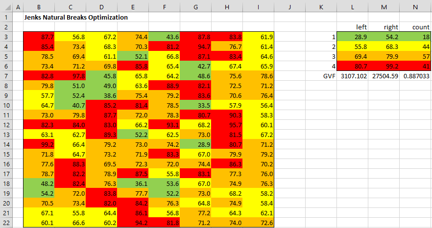
The Jenks Natural Breaks algorithm is commonly used to color maps as shown in Figure 8.

Figure 8 – Maps using Jenks Natural Breaks

Here, we use green for those cells in class 1, yellow for class 2, orange for class 3, and red for class 4 of Example 1. You can accomplish this using Excel’s conditional formatting capability. For example, to format the cells in category 1,

1. Highlight range B3:I22
2. Select Home > Styles|Conditional Formatting > New Rule…
3. In the New Formatting Rule dialog box, click on Use a formula to determine which cells to format
4. Under Format values where this formula is true, type the formula =AND(B3>=L3,B3<=M3)
5. Click the Format… button
6. In the Format Cells dialog box, click on the Fill tab, and choose the Green color
7. Click the OK button on this dialog and on the next dialog box that appears

You can repeat this procedure to format the other three classes.

References

EHDP (2015) Jenks natural breaks explained
https://www.ehdp.com/methods/jenks-natural-breaks-2.htm#:~:text=What%20is%20%22Natural%20Breaks%22%3F,should%20have%20the%20same%20color.

Excel Easy (2016) Conditional formatting
https://www.excel-easy.com/data-analysis/conditional-formatting.html