Basic Concepts
Suppose the variances of the residuals of an OLS regression are known, i.e. var(εi) = σi2. When we assume homogeneity of variances, then there is a constant σ such that σi2 = σ2 for all i. When this is not so, we can use WLS regression with the weights wi = 1/σi2 to arrive at a better fit for the data which takes the heterogeneity of the variances into account.
Note that in this case, an observation with a larger residual variance has a smaller weight and an observation with a smaller residual variance has a larger weight.
Examples
Example 1: A survey was conducted to compile data about the relationship between CEO compensation and company size. The summarized data from 200 respondents is shown in Figure 1. Create a regression model for this data and use it to predict the wages of a CEO for a company whose annual revenue is $200 million a year.
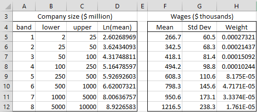
Figure 1 – Relationship between company size and CEO compensation
The companies were divided into eight bands, as shown in columns A through C of Figure 1: band 1 consists of companies whose revenues are between $2 million and $25 million, while band 8 consists of companies with revenues between $5 billion and $10 billion. The mean wages for the CEO’s in each band is shown in column F with the corresponding standard deviations shown in column G.
Our goal is to build a regression model of the form
wages = b0 + b1 ∙ LN(mean company size)
where LN(mean company size) for the 8 bands are shown in column D of Figure 1. E.g. the value in cell D5 is calculated by the formula =LN(AVERAGE(B5,C5)).
Dealing with unequal variances
Note that the standard deviations in column G, and therefore the variances, for the different bands are quite different, and so we decide not to use an OLS regression model, but instead we use a WLS model with the weights shown in column H of Figure 1. E.g. the value in cell H5 is calculated by the formula =1/G5^2. Here, we are using the sample data standard deviations si as an estimate for the population residual standard deviations σi.
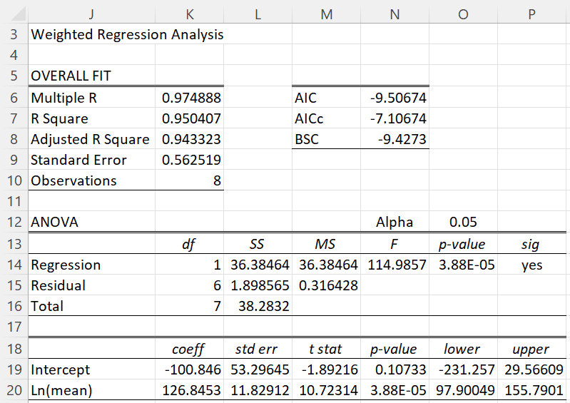
The WLS regression analysis is shown in Figure 2 using the approach described for Example 1 of WLS Regression Basic Concepts.
Figure 2 – Regression where the standard deviations are known
This model takes the form
wages = -100.846 + 126.8453 ∙ LN(mean company size)
Thus, the predicted average wages of a CEO in a company with $200 million in revenues is
wages = -100.846 + 126.8453 ∙ LN(200) = 571.221
This means that a CEO for a company with $200 million in revenues is estimated to earn $571,221 in wages.
Note that if instead of WLS regression, we had performed the usual OLS regression, we would have calculated coefficients of b0 = -204.761 and b1 = 149.045, which would have resulted in an estimate of $429,979 instead of $571,221.
Guidelines
Very seldom are the standard deviations known, but instead, need to be estimated from the residuals of OLS regression. Here are some guidelines for how to estimate the value of the σi. Once an estimate of the standard deviation or variance is made, the weights used can be calculated by wi = 1/σi2.
- If a residual plot against one of the independent variables has a megaphone shape, then regress the absolute value of the residuals against that variable. The predicted values of the residuals can be used as an estimate of the σi.
- If a residual plot against the y variable has a megaphone shape, then regress the absolute value of the residuals against the y variable. The predicted values of the residuals can be used as an estimate of the σi.
- If a plot of the squared residuals against one of the independent variables exhibits an upwards trend, then regress the squared residuals against that variable. The predicted values of the residuals can be used as an estimate of the σi2.
- If a plot of the squared residuals against the y variable exhibits an upwards trend, then regress the squared residuals against the y variable. The predicted values of the residuals can be used as an estimate of the σi2.
Note that usually, the WLS regression coefficients will be similar to the OLS coefficients. When this is not so, you can repeat the process until the regression coefficients converge, a process called iteratively reweighted least squares (IRLS) regression. We won’t demonstrate this process here, but it is used in LAD regression.
More Examples
Example 2
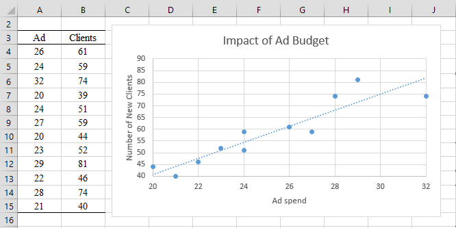
A marketing team is trying to create a regression model that captures the relationship between advertising expenditures and the number of new clients, based on the data in Figure 3.
Figure 3 – Impact of advertising budget on # of new clients
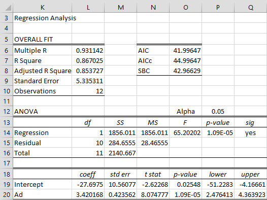
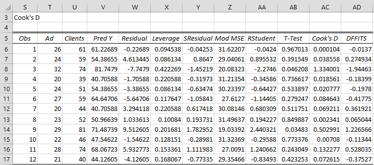
Using the Real Statistics Multiple Regression data analysis tool (with the X values from range A3:A15 and the Y values from range B3:B15), we obtain the OLS regression model shown in Figure 4 and the residual analysis shown in Figure 5.
Figure 4 – OLS regression analysis
Figure 5 – Residuals analysis
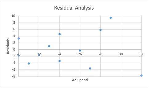
We now highlight range T6:T17, hold down the Ctrl key and highlight range W6:W17. Next, we select Insert > Charts|Scatter to obtain the chart in Figure 6 (after adding the axes and chart titles). This plot of the residuals versus the Ad values shows a slight megaphone pattern, which indicates a possible violation of the homogeneity of variances assumption.
Figure 6 – Chart of Ad Spend vs. Residuals
We could use the reciprocals of the squared residuals from column W as our weights, but we obtain better results by first regressing the absolute values of the residuals on the Ad spend and using the predicted values instead of the values in column W to calculate the weights.
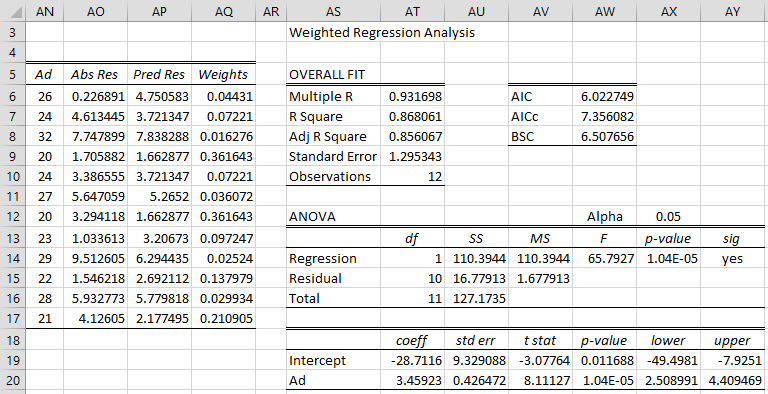
These weights are calculated on the left side of Figure 7. Here, cell AN6 contains the formula =T6, cell AO6 contains the formula =ABS(W6), range AP6:AP17 contains the array formula =TREND(AO6:AO17,AN6:AN17) and cell AQ6 contains the formula =1/AP6^2.
Next, we perform WLS regression using the X values from range A3:A15, the Y values from range B3:B15 (see Figure 3), and weights from range AQ6:AQ17. The result is shown on the right side of Figure 7.
Figure 7 – Weighted regression
Example 3
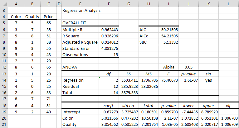
Repeat Example 1 of Least Squares for Multiple Regression with the data shown on the left side of Figure 8.
Figure 8 – OLS regression
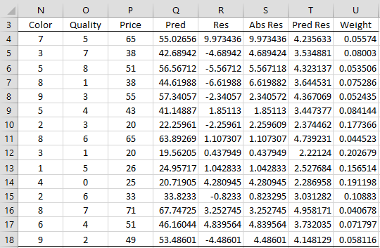
We next construct the table shown in Figure 9.
Figure 9 – Residual analysis
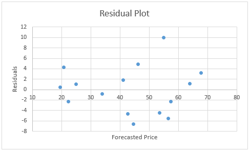
The forecasted price values shown in column Q and the residuals in column R are calculated by the array formulas =TREND(P4:P18,N4:O18) and =P4:P18-Q4:Q18. The scatter plot for the residuals vs. the forecasted prices (based on columns Q and R) is shown in Figure 10.
Figure 10 – Forecasted Price vs. Residuals
As in Figure 6, Figure 10 shows evidence that the variances are not constant. We now redo the analysis using WLS regression. We first use OLS regression to obtain a better estimate of the absolute residuals (as shown in column T of Figure 9). Next, we use these to calculate the weights (as shown in column U of Figure 9). E.g. range T4:T18 contains the array formula =TREND(ABS(R4:R18),Q4:Q18) and range U4:U18 contains the array formula =1/T4:U18^2.
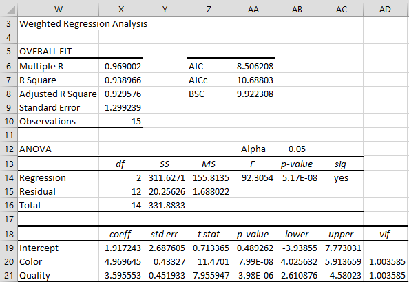
Finally, we conduct the Weighted Regression analysis using the X values in columns N and O, the Y values in column P and the weights in column U, all from Figure 9. The result is displayed in Figure 11.
Figure 11 – WLS regression
Example 4
A new psychological instrument has just been developed to predict the stress levels of people. The psychologist who developed this instrument wants to use regression to determine the relationship between the scores from this instrument and the amount of the stress hormone cortisol in the blood based on the data in columns A, B and C of Figure 12.
Figure 12 – Data for stress test
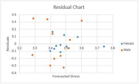
Here Males are coded by 1 and Females by 0. An OLS regression model is created and the residuals are calculated as shown in column R of Figure 12. A residuals chart is created from columns Q and R, as shown in Figure 13.
Figure 13 – Residuals chart
As we can see from the chart, the residuals for females are clustered in a narrower band than for males, (-.11, .17) vs. (-.32, .35). In fact, the variance of the residuals for men can be calculated by the formula =VAR.S(R14:R24), while the variance for women can be calculated by the formula =VAR.S(R4:R13). The corresponding weights used for men and women are the reciprocals of these values. These results are shown in Figure 14.
Figure 14 – Calculation of weights
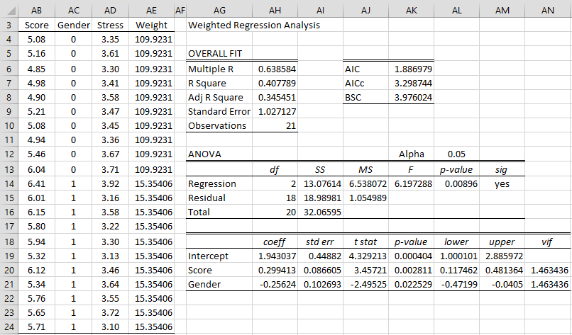
We now create the WLS regression analysis shown in Figure 15.
Figure 15 – WLS regression
Examples Workbook
Click here to download the Excel workbook with the examples described on this webpage.
References
Wikipedia (2018) Weighted least squares
https://en.wikipedia.org/wiki/Weighted_least_squares
Eisenhauer, J. G. (2003) Regression through the origin
https://onlinelibrary.wiley.com/doi/10.1111/1467-9639.00136
Huang, Y. (2021) Weighted least squares
No longer available online
Shalizi, C. (2015) Weighted and generalized least squares
https://www.stat.cmu.edu/~cshalizi/mreg/15/lectures/24/lecture-24–25.pdf


Hi, this is very confusing. Especially when I choose WLS in the Real Statistics option under multiple Regression and it indicates that the weights themselves need to be contained in 1 column; isn’t there a different weight for each of the regressors in the equation?
Hi Monica,
No, the weights are on the data not the regressors. If you have 5 regressors and 50 tuples of data then you have 50 weights. For more details see https://real-statistics.com/multiple-regression/weighted-linear-regression/weighted-regression-basics/
Charles