Approach
Given a set of n points (x11, …, x1k, y1), …, (xn1, …, xnk, yn), in ordinary least squares (OLS) the objective is to find coefficients b0, …, bk so as to minimize
where![]()
In weighted least squares, for a given set of weights w1, …, wn, we seek coefficients b0, …, bk so as to minimize
Using the same approach as that is employed in OLS, we find that the k+1 × 1 coefficient matrix can be expressed as
where W is the n × n diagonal matrix whose diagonal consists of the weights w1, …, wn.
The n × 1 matrix of predicted y values Y-hat = [ŷi] and the residuals matrix E = [ei] can be expressed as
An estimate of the variance of the residuals is given by
where dfRes = n – k – 1 and
It turns out that
as for OLS. Also, dfReg = k and dfT = n – 1, as for OLS. We will use definitions of SSReg and SST that are modified versions of the OLS values, namely
where 1 is the n × 1 column vector consisting of all ones. Note that
As for ordinary multiple regression, we make the following definitions
An estimate of the covariance matrix of the coefficients is given by
Note too that the values of the above formulas don’t change if all the weights are multiplied by a non-zero constant.
Example
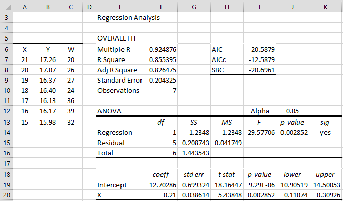
Example 1: Conduct weighted regression for that data in columns A, B, and C of Figure 1.
Figure 1 – Weighted regression data + OLS regression
The right side of the figure shows the usual OLS regression, where the weights in column C are not taken into account. Figure 2 shows the WLS (weighted least squares) regression output.
Figure 2 – Weighted least squares regression
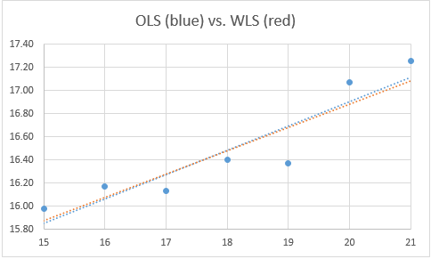
We see from Figure 3 that the OLS regression line 12.70286 + 0.21X and the WLS regression line 12.85626 + 0.201223X are not very different.
Figure 3 – Comparison of OLS and WLS regression lines
Key formulas
The formulas used to calculate the values in all the cells in Figure 2 are the same as those in Figure 1 with the following exceptions:
| Cells | Item | Formula |
| N19:N20 | coefficients | =MMULT(MINVERSE(MMULT(TRANSPOSE(DESIGN(A7:A13)),C7:C13* DESIGN(A7:A13))),MMULT(TRANSPOSE(DESIGN(A7:A13)),C7:C13*B7:B13)) |
| O19:O20 | std errors | =SQRT(DIAG(P15*MINVERSE(MMULT(TRANSPOSE(DESIGN(A7:A13)),C7:C13* DESIGN(A7:A13))))) |
| O16 | SSTot | =SUMPRODUCT(B7:B13^2,C7:C13)-SUMPRODUCT(B7:B13,C7:C13)^2/SUM(C7:C13) |
| O14 | SSReg | =SUMPRODUCT(C7:C13,MMULT(DESIGN(A7:A13),N19:N20)^2)-SUMPRODUCT(B7:B13,C7:C13)^2/SUM(C7:C13) |
Figure 4 – Key formulas in Figure 2
Note that the formulas in range N19:N20, range O19:O20, and cell O14 are array formulas, and so you need to press Ctrl-Shft-Enter (unless you are using a newer version of Excel that supports dynamic arrays, in which case you only need to press Enter).
Using weighted least-squares regression
Until now, we haven’t explained why we would want to perform weighted least squares regression. Generally, WLS regression is used to perform linear regression when the homogeneous variance assumption is not met (aka heteroscedasticity or heteroskedasticity). See WLS regression and heteroscedasticity.
Examples Workbook
Click here to download the Excel workbook with the examples described on this webpage.
References
Wikipedia (2018) Weighted least squares
https://en.wikipedia.org/wiki/Weighted_least_squares
Eisenhauer, J. G. (2003) Regression through the origin
https://web.ist.utl.pt/~ist11038/compute/errtheory/,regression/regrthroughorigin.pdf
Huang, Y. (2021) Weighted least squares
No longer available online
Shalizi, C. (2015) Weighted and generalized least squares
https://www.stat.cmu.edu/~cshalizi/mreg/15/lectures/24/lecture-24–25.pdf


May I know how did you plot the unweighted and weighted regression lines into one graph? I would like to visually compare the two regression lines as shown in Figure 3. Thank you.
You can download the spreadsheet that contains this graph from
https://real-statistics.com/free-download/real-statistics-examples-workbook/
You should download the Regression 1 workbook.
The steps that I used to create the graph are as follows
1. You start by highlighting A7:B13 and then selecting Insert>Charts|Scatter. This plots X vs Y.
2. Next add a linear trendline. This is done by clicking on any of the points in the chart and right clicking. Select the Add Trendline option in the menu that appears and then select Linear.
3. Next add the two points U16:U17 and V16:V17 to the chart. Here U16 and U17 contain the smallest and largest X values in column A. The corresponding Y values are specified by inserting the formula =N$19+N$20*U6 in cell V16, highlighting V16:V17, and pressing Ctrl-D. These are the y values for these points for the weighted regression.
4. These two points are added to the chart by clicking on the chart and selecting Chart Design>Data|Select Data, and clicking on the Add button and specifying U16:U17 as the X values and V16:V17 as the Y values.
5. Next click on either one of these points on the chart, and right click to add the linear trendline in the same manner as described above.
6. Finally, you need to remove the display of these two points from the chart (leaving only the trendline). This is done by double-clicking on one of these points to open the Format Data Point dialog box. Select the Pouring Bucket icon and then the Marker option. Next click on Fill and select No Fill.
Charles
The Adjusted R Square for the example above is calculated differently using the XRealStatistics add-in than how I expected and was described on the Multiple Correlation page (https://real-statistics.com/correlation/multiple-correlation/). I see the difference is in the numerator, where (n-1) is now just (n). Can you explain why the Adjusted R Square is calculated differently in this case?
The value calculated on the Multiple Correlation webpage should be the same as the calculation for (the unadjusted) R Square. The adjusted R Square is a refinement that can be used for either of these approaches.
Charles
I am struggle with code “DESIGN”. Excel stop working “=MMULT(MINVERSE(MMULT(TRANSPOSE(DESIGN(A2:A14)),C2:C14*DESIGN(A7:A13))),MMULT(TRANSPOSE(DESIGN(A2:A14)),C2:C14*B2:B14))” because of “DESIGN”. Excel pointed.
I would appreciate your help. Thank you.
Hi Misa,
The formula on the webpage is
=MMULT(MINVERSE(MMULT(TRANSPOSE(DESIGN(A7:A13)),C3:C13*DESIGN(A7:A13))),MMULT(TRANSPOSE(DESIGN(A7:A13)),C7:C13*B7:B13))
In your formula, you include the term DESIGN(A7:A13). This should probably be DESIGN(A2:A14). If you use A2:A14 in one place, you probably need to use A2:A14 (and similarly B2:B14 and C2:C14).
Charles
Thank you for your response and sorry for my miss typo. However, the Excel still did not work. I do not download ” Real Statistics Resource Pack” yet. Thank you for your help. =MMULT(MINVERSE(MMULT(TRANSPOSE(#NAME?(E2:E14)),F2:F14*DESIGN(E2:E14))),MMULT(TRANSPOSE(DESIGN(E2:E14)),F2:F14*B2:B14))
Hello Misa,
What is the cell reference that is causing Excel’s #NAME? error?
Charles
Hello, Charles.
I appreciate your help.
The Excel did not work these cells; N19:N20, O19:O20, O19:O20, O14 except for O16. Because O16 does not use the code “DESIGN” in the formula.
Thank you very much.
Hello Misa,
Does this mean that you now have it working?
Charles
Hello. Charles,
Unfortunately, they do not work so far… I do not find DESING code in Excel.
Thank you.
Misa,
DESIGN is not an Excel worksheet function. You need to have the Real Statistics Resource Pack installed to use it.
Charles
Hi, Charles,
Thank you very much,
I am using the weighted regression for the new lab data. How can I define the weights for the respective data set ?
Pawan,
You can use any weights that you like. It is entirely up to you. The weights you choose depend on what you are trying to accomplish. The Real Statistics website describes how to choose weights that correct for violations of assumptions.
Charles
I have a slightly different, but related, problem. Any advice would be most welcome.
I have test data yi, for known xi, and want to fit a user-chosen curve (e.g. linear for a start). However, I want to bias the result so that the sum of the abs(errors) in which the model underestimates the test data (“safe”) are larger than those in which it overestimates the test data (“unsafe”) by a user-selected factor. For example, one might choose to make 90% of the total error to be “safe”, and allow 10% to be “unsafe”. One can do it using the GRG solver to minimize the total error (taking sign into account), but that is slow, clunky and not very accurate (I guess the minimums are very flat). Also problem-dependent, I suspect. Is there a neat way to do it? The numerical experiments I have tried show that the slope of the fitted line is in all cases very close to the slope of the traditional linear regression line, but the offset changes depending on the weight factor chosen. Does that give any clues?
Hello John,
I don’t have a solution except via Solver, but perhaps the following paper would be helpful
https://www.jstor.org/stable/2286345
Charles
What would be the equations if the points varied in both the x and y direction (i.e., there was known uncertainty of the points in the y direction and in the x direction?
This is a different type of regression. You need to investigate Deming regression or Total Least Squares regression. See
https://www.real-statistics.com/regression/deming-regression/
https://www.real-statistics.com/regression/total-least-squares/
Charles
Hello! I am trying to regress on two x values – is there an easy way to modify this formula to get coefficients for that? The second X value is B2:B1030
=MMULT(MINVERSE(MMULT(TRANSPOSE(DEsign(A2:A1030)),C2:C1030*DEsign(A2:A1030))),MMULT(TRANSPOSE(DEsign(A2:A1030)),C2:C1030*D2:D1030))
I would think that you would replace A2:A1030 by the data for the two x values. If these data were stored in say E2:F1030, then replace A2:A1030 by E2:F1030.
Charles
Thank you so much Charles! this worked 🙂
Thank you for this great resource and the add-in!
Helped me out a lot!
Best wishes,
Josh
Hello,
I’m struggling to implement the formulas listed in Figure 4. Especially the DESIGN() function. I have downloaded your add-in, installed it just like it was described in the instruction (it is shown in ALT + T + I panel and also it is check-marked) but I’m still getting this #NAME? error while using formulas from Figure 4 or when viewing your example workbook. Can you tell me what is inside that DESIGN() function? I only need it from your set so there’s no need in fixing the add-in because the rest I have already handled.
Also when applying the formulas to the ranges (such as N19:N20) I have to select the range, type the formula and than press Ctrl + Shift + Enter? Or I can just select the first cell from a range and then press Ctrl + Shift + Enter and the formula will auto-expand to other cells?
Thanks in advance,
Fryderyk
Fryderyk,
What do you see when you enter the formula =VER() in any cell?
What version of Excel are you using?
Charles
Fryderyk,
What do you see when you enter the formula =VER() in any cell?
What version of Excel are you using?
Charles
=VER() gives a #NAME? error but when I opened the Account window it was stated there that I’m using this version:
Microsoft® Excel® for Microsoft 365 MSO (Version 2110 Build 16.0.14527.20234) 32-bit
Fryderyk,
This means that the Real Statistics add-in was not installed and so Excel doesn’t recognize any of the added functionality.
I suggest that you go back to the webpage from where you downloaded Real Statistics and follow the Installation instructions. If there is a problem, then please look at the Troubleshooting section.
Charles
OK, I tried to install it again (properly this time) and IT WORKED!
Thank you very much!
Thanks for sharing the good news.
Charles