Objective
On this webpage we provide the technical details, using calculus, for estimating the Tobit regression coefficients based on maximizing the log-likelihood function.
Log-likelihood function
As explained at Tobit Regression Model Description, the log-likelihood function for sample data is given by
The second equality follows from the first since when yi > 0
with xi0 = 1, and similarly when yi = 0.
Let γ = β/σ and θ = 1/σ. Thus
where
Recall that the pdf for the standard normal distribution can be expressed as
Thus
It now follows that
If n1 = the number of observations for which yi > 0 then
First derivatives
Since
it follows that
and so
Also
where
It now follows that
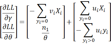
Thus, the gradient is
Second derivatives
First note that
Next note that

Also
It now follows that
Thus
Putting it all together, we get the Hessian matrix
Newton’s method
In general, Newton’s method provides an iterative approach for maximizing a function via
For Tobit regression, X is (γ, θ) and f(X) is LL viewed as a function of (γ, θ). Finally, ∇f and H are the gradient and Hessian, respectively. The formula for the gradient is shown at the end of the First Derivatives section above, and the Hessian is shown at the conclusion of the Second Derivatives section above.
Once we estimate the parameters γ, θ, we obtain estimates for β, σ via
σ = 1/θ βj = γjσ = γj/θ
We now use the delta method to estimate the standard errors. First note that
Now, define
Thus, the estimated asymptotic covariance matrix in terms of (β, σ) is equal to
The inverse of the Hessian matrix is a reasonable estimate of the covariance matrix in terms of (γ, θ), namely
Putting these together, we get the following estimate of the covariance matrix.
Thus, the square root of the items on the main diagonal of this matrix provides an estimate of the standard errors of the regression coefficients.
References
Shanaev, S. (2021) Tobit model explained: censored regression (Excel)
https://www.youtube.com/watch?v=QS3OAYML2nM
Munk-Nielson, A. (2016) The Tobit model
https://www.youtube.com/watch?v=IwsE8Rr6l6E
Demeritt, J. (2024) Tobit model
https://jdemeritt.weebly.com/uploads/2/2/7/7/22771764/tobit1.pdf
Greene, W. (2003) Econometric analysis. New Jersey: Prentice Hall.
Wikipedia (2024) Tobit model
https://en.wikipedia.org/wiki/Tobit_model
SAS (1999) Computing predicted values for a Tobit model
https://www.sfu.ca/sasdoc/sashtml/stat/chap36/sect24.htm
Olsen, R. J. (1978) Note on the uniqueness of the maximum likelihood estimator for the Tobit model
Greene, W. (2014) Censoring, Tobit and two part models
https://pages.stern.nyu.edu/~wgreene/DiscreteChoice/2014/DC2014-10-Censoring&Truncation.pdf


