LAD Regression using Simplex Method

Basic Concepts

Using the Simplex method, we turn the problem of finding the minimum of the absolute deviations between the observed values of y and the predicted values of y.

into the linear programming problem of minimizing subject to the constraints

for all i = 1, …, n.

We can use Excel’s Solver to solve this linear programming problem, employing the Simplex Linear Programming method, where each data element results in two constraints.

Example Setup

Example 1: Repeat Example 1 of Least Squares for Multiple Regression using LAD regression.

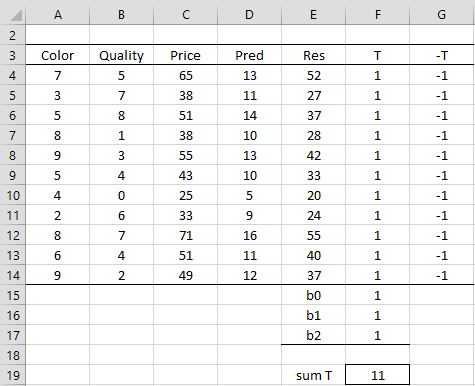
We repeat the data from Example 1 in range A3:E14 of Figure 1 along with the setup required for using Excel Solver’s Simplex method.

Figure 1 – Data and set up for Simplex method

Here, cell D4 contains the formula =$F$15+MMULT(A4:B4,$F$16:$F$17), E4 contains =C4-D4, G4 contains =-F4 and F19 contains =SUM(F4:F14). The cells in range F4:F14 that represent the t_i are set to initial guesses of 1 as are the regression coefficients in range F15:F17. We could replace these guesses with some other values. Note that we place the coefficient cells right below the t_i cells so that we have a contiguous range of cells that will be changed during the running of the Solver algorithm.

Solver

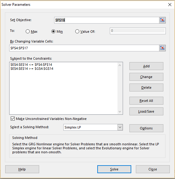
We now select Data > Analysis|Solver and fill in the dialog box that appears as shown in Figure 2.

Figure 2 – Solver dialog box

Note that we want to minimize the value in cell F19, which will contain the sum of the absolute value of the deviation between the observed y values (column C) and those predicted by the regression model (column D). The minimization is carried out by varying the values in the range F4:F14, which contain the absolute deviations, as well as range F15:F17, which contains the regression coefficients.

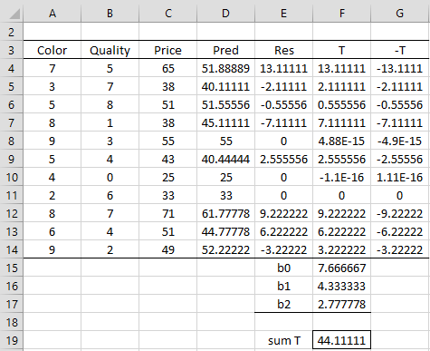
We specify the constraints for the optimization process in the usual way, except that this time we combine constraints such as E4 <= F4, E5 <= F5, E6 <= F6, …, E14 <= F14 by using a range inequality E4:E14 <= F4:F14. Finally, we request the use of the Simplex LP method. When we press the OK button, we get the results shown in Figure 3.

Figure 3 – LAD Regression results

The LAD regression model is

Price = 7.667 + 4.333 * Color + 2.778 * Quality

Since we have two independent variables, as noted previously, at least three data elements will have zero residual, namely those in rows 8, 10, and 11.

One problem with using the Simplex method in Excel is that it is limited to 100 constraints, which means that it will only support LAD models with at most 50 data elements.

References

Wikipedia (2016) Least absolute deviations
https://en.wikipedia.org/wiki/Least_absolute_deviations

Wikipedia (2016) Simplex algorithm
https://en.wikipedia.org/wiki/Simplex_algorithm

Cheusheva, S. (2021) How to use Solver in Excel with examples
https://www.ablebits.com/office-addins-blog/2016/06/22/how-to-use-solver-in-excel-with-examples/