Introduction
Whereas the Durbin-Watson Test is restricted to detecting first-order autoregression, the Breusch-Godfrey (BG) Test can detect autocorrelation up to any predesignated order p. It also supports a broader class of regressors (e.g. models of the form yi = axi + byi-1 + c).
Approach
The test is carried out as follows:
Step 1: Run OLS regression to calculate an estimate of the model
![]() and find the residuals e1, e2, …, en
and find the residuals e1, e2, …, en
Step 2: Using these sample residuals e1, e2, …, en, run an OLS regression for the model
Step 3: We now test the null hypothesis
Based on this null hypothesis, If the sample size is sufficiently large, then
LM = nR2 ∼ χ2(p)
where n is the original sample size and R2 is the value calculated in step 2. If p-value < α, then the null hypothesis is rejected, and so at least one of the pj is significantly different from zero.
The test statistic nR2 is sometimes called the LM (Lagrange multiplier) statistic. There is an F test version of the Breusch-Godfrey test that uses a modified version of this statistics LM*.
where k = the number of independent variables. Note that dfRes from the regression in step 2 is equal to n – p – k – 1.
If p = 1, the BG test tests for first-order autoregression and is also called Durbin’s M test.
Commonly used estimates for p are .75 × n1/3 or 4 × (n/100)2/9.
Example
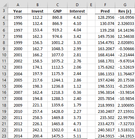
Example 1: Figure 1 shows the Interest Rate, GDP and Investment Volume for a certain country in the years 1995 through 2014. The financial analysts want to use the Interest Rate and GNP to forecast future Investment Volume based on a linear regression model. Determine whether there is 4th-order autocorrelation using the Breusch-Godfrey test (ignoring the fact that the sample is not particularly large).
Figure 1 – Investment volume vs. GDP and Interest Rate
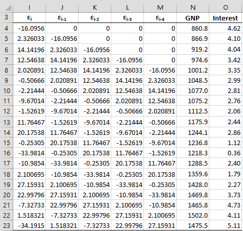
The predicted values of Invest are displayed in column F. The values in range F4:F23 can be calculated using the array formula =TREND(B4:B23, C4:D23) and the residuals in range G4:G23 can be calculated by the array formula =B4:B23-F4:F23. We now perform the regression described in Step 2 using the data for the dependent variable shown in range I4:I23 of Figure 2 and the data for the independent variables shown in range J4:O23.
Figure 2 – Data for Step 2 in the Breusch-Godfrey test
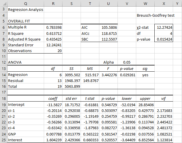
The results of this regression (using the Multiple Linear Regression data analysis tool) are shown in Figure 3.
Figure 3 – Breusch-Godfrey test results
We have also added the calculation of the Breusch-Godfrey test in the upper right side of Figure 3. The BG statistic (cell X6) is calculated by the formula =R7*(R10-X7), df (cell X7) is calculated by =COUNTA(J3:M3) and the p-value of the test (cell X8) is calculated by =CHISQ.DIST.RT(X6,X7).
We see that p-value = .0154, which indicates that there is autocorrelation for some order less than or equal to 4.
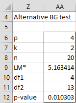
The modified version of the test is shown in Figure 4.
Figure 4 – LM* test
Worksheet Functions
Real Statistics Functions: The following functions are available in the Real Statistics Resource Pack.
BGSTAT(R1, R2, p, chi) = the Breusch-Godfrey LM statistic for the X data in R1 and Y data in R2, when chi = TRUE (default); otherwise the LM* statistic is returned
BGTEST(R1, R2, p, chi) = the p-value of the Breusch-Godfrey LM test for the X data in R1 and Y data in R2 for order p when chi = TRUE (default); otherwise the p-value of the LM* test is returned
If p is omitted it defaults to 1.
For Example 1, the result from the formula =BGSTAT(C4:D23,B4:B23,4) is the value shown in cell X6 and the result from the formula =BGTEST(C4:D23,B4:B23,4) is the value shown in cell X8. Note that the results from the formula =BGTEST(C4:D23,B4:B23,3) is .0344, while BGTEST(C4:D23,B4:B23,2) = .113 and BGTEST(C4:D23,B4:B23,1) = .200. This indicates that there is third order autocorrelation, but not first or second order autocorrelation.
For Example 1, the formula =BGSTAT(C4:D23,4,FALSE) returns the value shown in cell AA9 and the formula =BGSTAT(C4:D23,4,FALSE) returns the value shown in cell AA12.
Note too that the Durbin-Watson test is inconclusive for first-order correlation (D-stat = 1.218, with DLower = 1.100 and DUpper = 1.537).
Data Analysis Tool
See Breusch-Godfrey and Newey-West Tool for information about how to perform the Breusch-Godfrey test using the Real Statistics Breusch-Godfrey and Newey-West data analysis tool.
Examples Workbook
Click here to download the Excel workbook with the examples described on this webpage.
References
Wikipedia (2018) Breusch-Godfrey test
https://en.wikipedia.org/wiki/Breusch%E2%80%93Godfrey_test
Wooldridge, J. M. (2013) Introductory econometrics, a modern approach (fifth edition). Cengage Learning
https://faculty.cengage.com/works/9781337558860
Stack Exchange (2015) Breusch-Godfrey test and the length of the lag, p
https://stats.stackexchange.com/questions/178813/breusch-godfrey-test-and-the-length-of-the-lag-p


