Objective
We describes how to use the Real Statistics Coarsened Exact Matching data analysis tool using an example.
See Real Statistics Support for CEM for a description of various Excel worksheet functions that are used by this data analysis tool.
Example
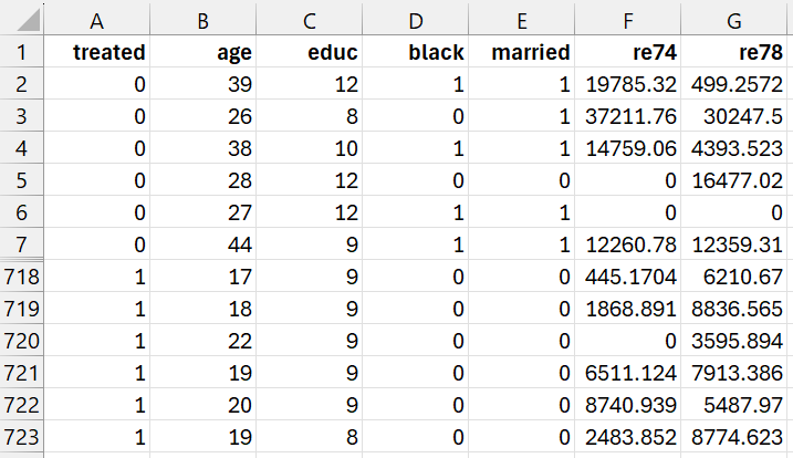
Example 1: The goal of the Lalonde study (1986) was to examine the effect of a job training program on real 1978 earnings. We will use the data shown in Figure 1 (a subset of the complete data). Here, only 12 rows of the data with 722 rows are displayed. 297 subjects received the job training (1 in column A) and 425 subjects did not receive the training (0 in column A). The data is arranged so that data for the control group precede those for the training group in Figure 1.
This is the same example as that used in PSM Example.
The subjects in this study were not randomly assigned to the treatment and control groups. Despite this, we want to use CEM to prune the data so that we can still determine how effective the treatment was in increasing 1978 revenues.
Here the data in columns B through F contain data for any confounding variables or variables that might be associated with whether a subject is in the treatment group or not. These variables are age, education (# of years in school), black (1 = black, 0 = not black), married (1 = married, 0 = not married), re74 (revenues in 1974). Finally, column G contains the outcome variable (revenues in 1978).
A link to the data set used is shown towards the end of this webpage.
Figure 1 – Lalonde study data
Coding
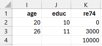
As explained in Real Statistics Support for CEM, we need to code the various variables as part of the coarsening process. For Example 1, we use the coding shown in Figure 2.
Figure 2 – CEM Coding
This means that we use the codes shown in Figure 2a.
| Variable | Code | Meaning | |
| age | 1 | age ≤ 20 yrs | |
| 2 | 20< age ≤ 26 | ||
| 3 | age > 26 | ||
| educ | 1 | educ ≤ 10 yrs | |
| 2 | educ = 11 | ||
| 3 | educ > 21 | ||
| re 74 | 1 | revenue = $0 | |
| 2 | $0< rev ≤ $3,000 | ||
| 3 | $3,000< rev ≤ $10,000 | ||
| 4 | rev > $10,000 | ||
| black | 0 | not black | |
| 1 | black | ||
| married | 0 | not married | |
| 1 | married |
Figure 2a – CEM Coding Explained
Accessing the data analysis tool
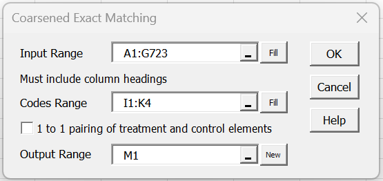
To conduct the analysis, press the Ctrl-m key combination to access the Real Statistics main menu. Next choose the Coarsened Exact Matching option from the Misc tab, and fill in the dialog box that appears as shown in Figure 3.
Figure 3 – CEM dialog box
Coarsening
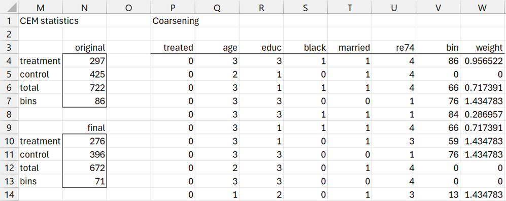
After clicking the OK button on the dialog box, initially the results shown in ranges M1:N6 and P1:U725 of Figure 4 appear (only the first 11 of 722 entries for range P3:U725 are displayed).
Figure 4 – CEM output (part 1)
We see from range N4:N6 of Figure 4 that Figure 1 contains data for 297 subjects in the treatment group and 425 subjects in the control group, for a total of 722 subjects.
The data in range P3:U725 shows the coarsening of the corresponding data in range A1:F723 of Figure 1, as calculated by the array formula =CEM_Coding(A1:F723,I1:K4).
For example, the first data row from Figure 1 contains the data for a subject in the control group with age = 39, educ = 12, black = 1, married = 1, re 74 = 19,785.32. Using the coding in Figure 2 or 2a, this results in a coding of age = 3, educ = 3, black = 1, married = 1, re74 = 4, exactly as shown in range Q4:U4 of Figure 4.
Bin signatures
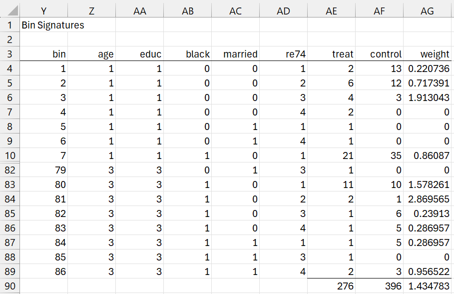
The data analysis tool next returns the output shown in range Z4:AD89 of Figure 5 using the array formula =SortsRowsUnique(Q429:U725). Only the first 7 and last 8 of 86 bin signatures are displayed.
Figure 5 – CEM output (part 2)
These are the only 86 rows that match with some treatment row in the data from Figure 4. This is why cell N7 from Figure 3 contains the value 86.
For example, the last row in Figure 5 (i.e. Z89:AD89) matches with the first row from Figure 4 (i.e. Q4:U4), which is why cell V4 contains the bin signature index of 86. In fact, there are 2 treatment rows with this bin signature (namely rows 432 and 440) and 3 control rows with this bin signature (namely rows 4, 61, and 76). This is why cell AE89 contains the value 2 and cell AF89 contains the value 3. We will come back to this shortly.
First, we note that the data analysis tool fills in column V of Figure 4 with signature indices for all the rows in Figure 4. This can be done by inserting the formula =RowMatch(Z$4:AD$89,Q4:U4) in cell V4, highlighting range V4:V725, and then pressing Ctrl-D.
Pruning based on bin signatures
As noted above, cell AE89 contains the value 2 and cell AF89 contains the value 3. In fact, cell AE4 contains the formula =COUNTIF(V$429:V$725,Y4) and cell AF4 contains the formula =COUNTIF(V$4:V$428,Y4). Highlighting range AE4:AF89 and pressing Ctrl-D fills in all the values in columns AE and AF as shown in Figure 5.
We see from cell AF90 in Figure 5, the total number of matching control group rows is 396, as calculated via the formula =SUM(AF4:AF89). The other 425 – 396 = 29 subjects in the treatment group are pruned since they don’t match any of the treatment group subjects.
Since the bin signatures in Figure 5 are based on the patterns of treatment rows from Figure 4, not surprisingly, all of the entries in column AE are positive counts. Many of the elements in column AF, however, contain zeros, which means that there are no subjects from the control group that have that bin signature, and therefore match the corresponding subject(s) from the treatment group with that bin signature. Since there is no match, treatments with a zero entry in column AF also need to be pruned.
This means that the total number of matching treatment subjects is 276 (cell AE90) as calculated by =SUMIF(AF4:AF89,”>0″,AE4:AE89). The other 297 – 276 = 21 treatment subjects are also pruned.
The revised number of treatment and control subjects is 297 and 396, for a total of 693. Of the original 86 bin signatures, 15 contain a zero in column AF, and so 71 bin signatures, as calculated by the formula =COUNTIF(AF4:AF89,”>0″), have matches. These are the values shown in range N10:N13 of Figure 4.
Assigning Weights
As described in Coarsened Exact Matching the weight for each subject in the treatment group is either 0, if they have been pruned, or 1 if there is a match. For the subjects in the control group, with bin signature b, the weight is calculated by the formula
The ratio nC/nT = 396/276 = 1.434783, as shown in cell AG90 of Figure 5. The weights for all the subjects in the control group are as shown in column AG. These can be calculated by placing the formula =IFERROR(AE4/AF4*AG$90,0) in cell AG4, highlighting range AG4:AG89, and pressing Ctrl-D.
Finally, we need to transfer these weights back to column W of Figure 4. This can be done by inserting the formula =IF(V4=0,0,INDEX(AG$4:AG$89,V4)) in cell W4, highlighting the W4:W428, and pressing Ctrl-D for the control rows. And then inserting the formula =IF(INDEX(AG$4:AG$89,V429)=0,0,1) in cell W429, highlighting the W429:W725, and pressing Ctrl-D for the treatment rows.
Pruning/weighting of the original data
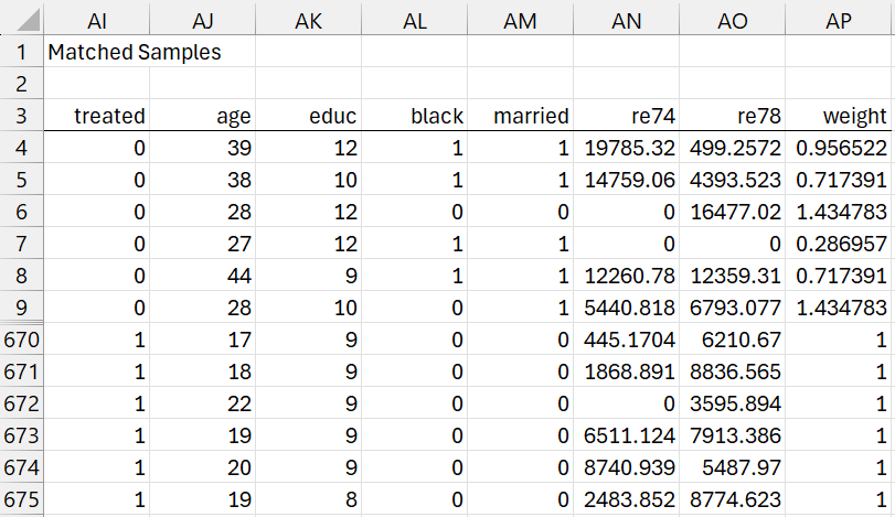
We now transfer the weights to the original (uncoarsened) data and prune any row with a zero weight. This is done via the array formula =Pruning(A1:G723,W3:W725), as shown in Figure 6 (only the first and last 6 rows are displayed). Here we also include the outcome variable re 78.
Figure 6 – CEM output (part 3)
Match Quality
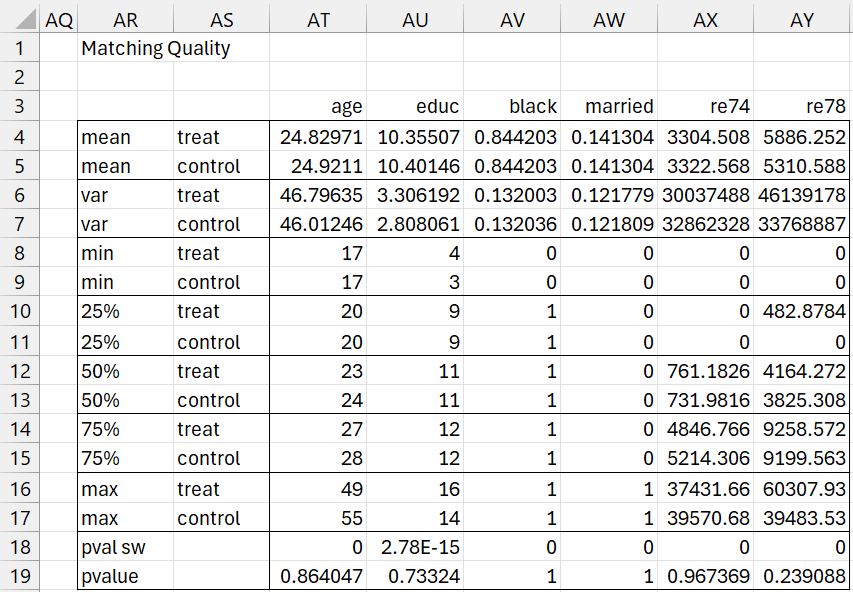
Just as we did for Propensity Score Matching, we can gauge the quality of the matching using the array formula =MatchQuality(AI3:AP675,FALSE). The output is shown in Figure 7.
Figure 7 – CEM output (part 4)
We see pretty good matching for all five confounding variables (age, educ, black, married, re 74). Note that the p-values shown in row 19 come from using weighted regression, as described in Figure 2 of Coarsened Exact Matching.
The only problem here is that weighted linear regression assumes normality of residuals, an assumption that fails since the Shapiro-Wilk p-values in row 18 are all zero. Since we don’t have a weighted non-parametric test, we’ll hope for the best with the data we have. In particular, we see evidence (p-value = .239088) that there isn’t a significant difference in 1978 revenues between the subjects in the treatment group, who received special training, and those in the control group who did not.
Test using Weighted Regression
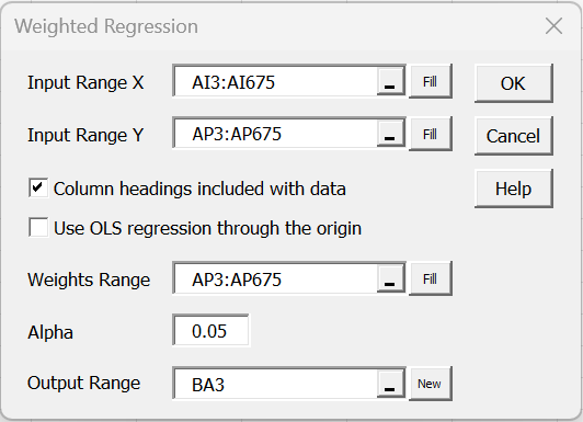
Using the matched data from Figure 6, we conduct the weighted regression using the dialog box shown in Figure 8.
Figure 8 – Weighted Regression Dialog Box
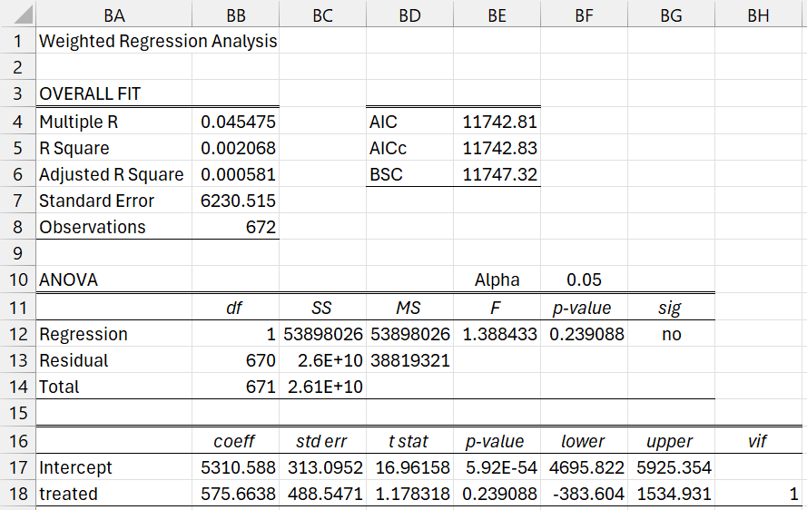
The results are shown in Figure 9.
Figure 9 – Weighted Regression Results
We see that the weighted difference for re78 between the treatment and control groups is 575.6638 (treated coefficient) and the weighted mean for the control group is 5310.588 (intercept). Thus, the weighted mean for the treatment group is 5310.588 + 575.6638 = 5886.25161. Since p-value = 0.239088, there isn’t a significant difference between the two groups.
Using the 1-to-1 option
As shown in Figure 3, the Coarsened Exact Matching data analysis tool provides a 1 to 1 pairing of treatment and control elements option (no weights). Click here for an example of how to use this option.
Examples Workbook
Click here to download the Excel workbook with the examples described on this webpage.
Links
References
King, G. (2015) Why propensity scores should not be used for matching
https://www.youtube.com/watch?v=rBv39pK1iEs
Huntington-Klein, N. (2012) Coarsened exact matching and entropy balancing
https://www.youtube.com/watch?v=M6AsS4zaWQk
Blackwell, M., Iacus, S., King, G., Porro, G. (2011) CEM for SPSS
https://projects.iq.harvard.edu/cem-spss/pages/how-use-cem-spss
Huffman, A. (2017) CEM: Coarsened exact matching explained
https://medium.com/@devmotivation/cem-coarsened-exact-matching-explained-7f4d64acc5ef
Wu, W. (2023) Coarsened exact matching
https://cem-linearinf.readthedocs.io/en/latest/tuto_cem.html
Wu, W. (2023) Balance checking
https://cem-linearinf.readthedocs.io/en/latest/tuto_balance.html
Wu, W. (2023) Inference
https://cem-linearinf.readthedocs.io/en/latest/tuto_inf.html
Wu, W. (2023) Sensitivity analysis
https://cem-linearinf.readthedocs.io/en/latest/tuto_sen.html
