Basic Concepts
To determine whether there is a significant difference between the effect on two groups (e.g. a treatment group and a control group), we normally randomly select a sample from the population being studied and then randomly assign subjects in the sample to the two groups. This is called an experimental study.
Sometimes it is impossible or unethical to randomly assign subjects to the two groups. For example, when studying the effects of smoking, we can’t assign non-smokers to the smoking group, and so there is no random assignment. The goal of experimental design is to reduce the chances that confounding variables will influence the outcome of the study. This is achieved since the random assignment of the sample groups tends to eliminate the effects of confounding variables.
When there is no random assignment of the sample into groups, then we have an observational study. We now need to take confounding variables explicitly into account. One approach for doing this is called coarsened exact matching (CEM), in which we identify all important confounding variables, and then determine matching subjects from the sample based on similar confounding variable values, pruning non-matching pairs.
Objective
In this way, we explicitly eliminate the effects of the confounding variables (instead of counting on the random assignment to accomplish this).
Coarsened Exact Matching is a technique that attempts to balance the impact of confounding factors on the two groups so that we can draw conclusions about the impact of a treatment on the outcome using observational data.
Essentially it is a preprocessing algorithm for converting observational data into quasi-experimental data, thereby removing baseline differences so that you can effectively compare treatment and control groups.
Comparison with Propensity Score Matching
Propensity Score Matching is another commonly used approach for matching in an observational study. Generally, CEM is the preferred approach. Its advantage is that we use the data from the actual confounding variables and not just the propensity score as a sort of summary of these variables.
Binning
As for Propensity Score Matching, CEM matches subjects in the treatment group with subjects in the control group based on confounding variables (which we can think of as properties). For each such property you need to coarsen the data values into discrete bins (as for a histogram). The more bins, the more data is required for the procedure to be effective. Subjects in each group are assigned a bin signature which represents the bin assignment for each property for that subject. Subjects in the two groups with exactly the same bin signature are matched.
For example, the age property can be binned as 0 = 0-20, 1 = 21-40, 2 = 41-60, 3 = 60+. Gender can be binned as 0 = female and 1 = male (and if necessary 2 = other). If these are the only properties, then there are 4 × 2 = 8 possible bin signatures: (0,0), (0,1), (1,0), …, (3,0), (3,1).
Weights
Because there will likely be an imbalance in the size of the treatment and control groups, weighting is used to balance the data.
Let B = the set of all matched bin signatures. We now show how to assign weights.
All unmatched elements in the treatment or control group are assigned a weight of zero, and so are excluded from the revised treatment and control groups.
All matched subjects in the treatment group are assigned a weight of 1.
For each bin signature b in B, define
Now define
Finally, define the weight for a subject b in the control group as
where nC = the total number of matched subjects in the control group and nT = the total number of matched subjects in the treatment group.
Example
Let’s suppose that only three bin signatures have matches where
- Bin 1: matched 2 treatment and 10 control subjects
- Bin 2: matched 4 treatment and 2 control subjects
- Bin 3: matched 6 treatment and 6 control subjects
Thus, nC = 10 + 2 + 6 = 18 and nT = 2 + 4 + 6 = 12, and so
Testing
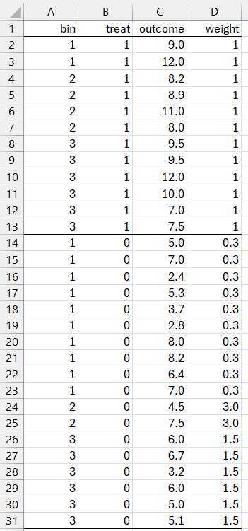
For this simple example, the results from CEM are as shown in Figure 1.
Figure 1 – CEM Output
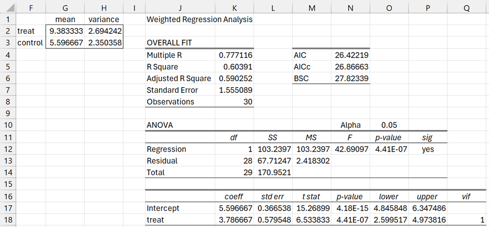
We first observe that the weighted means and variances for the treatment and control groups are as shown on the left side of Figure 2. Cell G2 is calculated by =MEAN(C2:C13,D2:D13), cell C3 by =MEAN(C14:C31,D14:D31), cell H2 by =WVAR(C2:C13,D2:D13), and cell H3 by =WVAR(C14:C31,D14:D31).
The mean for the treatment group is bigger than the mean for the control group. We now perform weighted regression to determine whether there is a significant difference between the two groups. This was done using Real Statistics’ Weighted Regression data analysis tool, as shown on the right side of Figure 2, with the X data B1:B31 from Figure 1, the Y data C1;C31 and the weights D1:D31.
Figure 2 – Weighted Linear Regression
We see from cell K18 that the difference between the groups is 3.786667, which is significant since p-value = 4.41E-07 (cell N18).
Real Statistics Support
Click here for a description of the Real Statistics worksheet functions and data analysis tool that supports CEM.
Click here for an example of how to use the Real Statistics Coarsened Exact Matching data analysis tool with weights in Excel.
Finally, click here for an example of how to use the Real Statistics Coarsened Exact Matching data analysis tool with the 1-to-1 option (without weights).
Examples Workbook
Click here to download the Excel workbook with the examples described on this webpage.
Links
References
King, G. (2015) Why propensity scores should not be used for matching
https://www.youtube.com/watch?v=rBv39pK1iEs
Huntington-Klein, N. (2012) Coarsened exact matching and entropy balancing
https://www.youtube.com/watch?v=M6AsS4zaWQk
Blackwell, M., Iacus, S., King, G., Porro, G. (2011) CEM for SPSS
https://projects.iq.harvard.edu/cem-spss/pages/how-use-cem-spss
Huffman, A. (2017) CEM: Coarsened exact matching explained
https://medium.com/@devmotivation/cem-coarsened-exact-matching-explained-7f4d64acc5ef
Wu, W. (2023) Coarsened exact matching
https://cem-linearinf.readthedocs.io/en/latest/tuto_cem.html
Wu, W. (2023) Balance checking
https://cem-linearinf.readthedocs.io/en/latest/tuto_balance.html
Wu, W. (2023) Inference
https://cem-linearinf.readthedocs.io/en/latest/tuto_inf.html
Wu, W. (2023) Sensitivity analysis
https://cem-linearinf.readthedocs.io/en/latest/tuto_sen.html


