Saturated model for two-way contingency tables

We begin by investigating the saturated model, which accounts for all the possible variables. We do this by reexamining Example 2 of Independence Testing using a log-linear approach.

Example

Example 1: Create a saturated log-linear model for the data in Example 2 of Independence Testing

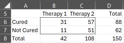
The data for the 150 patients are again summarized in the contingency table in Figure 1.

Figure 1 – Contingency table

Define the following coding of the categorical variables:

t₁ = 1 if therapy 1 and = -1 if therapy 2
t₂ = 1 if cured and = -1 if not cured

Based on this coding the data can be expressed as in Figure 2.

Figure 2 – Fitting the data to the saturated model

The log-linear model takes the form:

ln y_i = β₀ + β₁t_i1 + β₂t_i2 + β₃t_i1t_i2 + ln ε_i

Here all the variables are included, including the interaction terms. This is called the saturated model. We now find the values of the population coefficients β₀, β₁, β₂, β₃. As usual, using the sample data we find the estimates of these coefficients b₀, b₁, b₂, b₃, where

ln y_i = b₀ + b₁t_i1 + b₂t_i2 + b₃t_i1t_i2

It then follows (using the data in Figure 2) that:

3.434 = ln 31 = ln y₁ = b₀ + b₁⋅1 + b₂⋅1 + b₃⋅1 = b₀ + b₁ + b₂ + b₃

2.398 = ln 11 = ln y₂ = b₀ + b₁⋅1 + b₂(-1) + b₃(-1) = b₀ + b₁ – b₂ – b₃

4.043 = ln 57 = ln y₃ = b₀ + b₁(-1) + b₂⋅1 + b₃(-1) = b₀ – b₁ + b₂ – b₃

3.932 = ln 51 = ln y₄ = b₀ + b₁(-1) + b₂(-1) + b₃⋅1 = b₀ – b₁ – b₂ + b₃

Adding all four equations and dividing by 4 we get

b₀ = (ln 31 + ln 11 + ln 57 + ln 51)/4 = (3.434 + 2.398 + 4.043 + 3.932)/4 = 3.452

Adding the first two equations and dividing by 2 we get

b₁ = (ln 31 + ln 11)/2 – b₀ = (3.434 + 2.398)/2 – 3.452 = -.536

Now, adding the first and third equations and dividing by 2 we get

b₂ = (ln 31 + ln 57)/2 – b₀ = (3.434 + 4.043)/2 – 3.452 = .287

Adding the first and last and dividing by 2 we get

b₃ = (ln 31 + ln 51)/2 – b₀ = (3.434 + 3.932)/2 – 3.452 = .231

Thus the model is

ln y = 3.452 – .536 t₁ + .287 t₂ + .231 t₁t₂

which is equivalent to

y = exp(3.452 – .536 t₁ + .287 t₂ + .231 t₁t₂)

 

which is, in turn, is equivalent to

Using , the log-linear model takes the form (dropping the error term):

Marginal averages

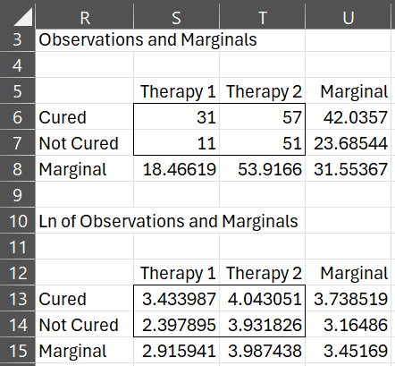
In Figure 3 we provide the contingency table for the logs of the original data in range S13:T14, but this time instead of calculating the marginal totals, we calculate the marginal averages.

Figure 3 – Marginal averages

Thus, for example, the marginal average for the Cured row (cell U13) contains the formula =AVERAGE(S13:T13) and the marginal average for the Therapy 1 column (cell S15) contains the formula =AVERAGE(S13:S14).

Note that b₀ = the grand mean (cell U15), b₁ = the mean for Cured (cell U13) minus the grand mean, b₂ = the mean for Therapy 1 (cell S15) minus the grand mean and b₃ = Cured × Therapy 1 (cell S13) minus the mean for Cured minus the mean for Therapy 1 plus the grand mean.

We now map the log values back into the original contingency table (range R5:U8) by using the exponential function. Thus the marginal average for the Cured row in the original contingency table (cell U6) is EXP(U13) = EXP(3.738519) = 42.0357. Note, however, that the arithmetic mean of 31 and 57 is not 42.0357. It turns out, however, that the geometric mean of 31 and 57 is 42.0357. Thus we could also put the formula GEOMEAN(S6:T6) in cell U6 and get the same value of 42.0357. This relationship is also true for the other marginal averages.

Observation

The saturated model is an exact fit for the data (i.e. the error terms are zero), and simply provides a new way of looking at the observed data.

The exact version of the coefficients calculated depends on the coding of the dummy variables used. E.g., if we use the coding

t₁ = 0 if therapy 1 and = 1 if therapy 2
t₂= 0 if not cured and = 1 if cured

then the log-linear regression model becomes:

ln y = 2.398 + 1.534 t₁ + 1.036 t₂ – .925 t₁t₂

Examples Workbook

Click here to download the Excel workbook with the examples described on this webpage.

Reference

Howell, D. C. (2010) Statistical methods for psychology (7^th ed.). Wadsworth, Cengage Learning.
https://labs.la.utexas.edu/gilden/files/2016/05/Statistics-Text.pdf