Basic Concepts
The homogeneous association model for (AB, BC, AC) consists of the saturated model with the λABC term dropped. It therefore has (a – 1)(b – 1)(c – 1) degrees of freedom. For Example 1 of Three-way Contingency Tables this is (2 – 1)(2 – 1)(3 – 1) = 2 degrees of freedom.
For this model, there is no easy formula for calculating the expected frequencies. We must use the iterative approach that is described in Iterative Proportional Fitting Procedure (IPFP).
Example
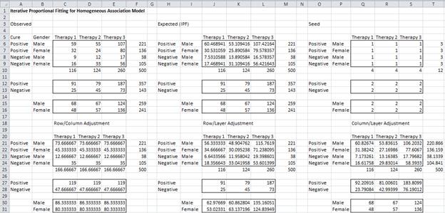
The first step of this iteration for Example 1 of Three-way Contingency Tables is shown in Figure 1.
Figure 1 – Finding expected freq for homogeneous association
Range A5:F16 displays the observed frequencies. H3:M16 displays the expected frequencies, which is the output of the iterative proportional fitting procedure. Range O3:T16 displays the initial values for the iteration (the seed values). To get the desired expected frequencies all the seed values need to be set to 1.
Range A20:F31 provides the output for the first row/column adjustment (to the seed values), range H20:M31 provides the output for the first row/layer adjustment and range O20:T31 provides the output to the first column/layer adjustment. The procedure continues until values in the marginal totals are sufficiently close to the marginal totals of the observed frequencies (these steps are not displayed in Figure 1).
From the expected frequencies, we obtain a χ2 (maximum likelihood) of .674, which with 2 degrees of freedom is not significant. Thus we conclude that this model is a good fit for the data.
Finally, note the following:
![]()
![]()
for any values of i, j, k, i′, j′, k′. E.g. the formulas =J57*K58/(J58*K57) and =J59*K60/(J60*K59) both have value .9655.
Examples Workbook
Click here to download the Excel workbook with the examples described on this webpage.
Reference
Howell, D. C. (2010) Statistical methods for psychology (7th ed.). Wadsworth, Cengage Learning.
https://labs.la.utexas.edu/gilden/files/2016/05/Statistics-Text.pdf
