Varimax Algorithm

Basic Concepts

As observed in Rotation, we seek an m × m orthogonal rotation U = [u_ij] of the factor matrix such that the rows represent the existing factors and the columns represent the new factors. The most popular rotation approach is called Varimax, which maximizes the differences between the loading factors while maintaining orthogonal axes. Varimax attempts to maximize the value of V where

The algorithm used is iterative and consists of the following steps. We illustrate each step using starting with the loading factors matrix from Figure 2 of Determining the Number of Factors.

Step 0

Normalize the loading factors matrix so that each row in the resulting matrix is a unit vector. This is done as usual by dividing each cell by the square root of the sum of squares in that row.

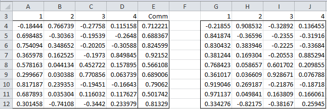
Figure 1 – Normalization of the Loading Factors matrix 

Range A4:D12 contains the original loading factors. The communalities are listed in column E. For example, cell E4 contains the formula =SUMSQ(A4:D4). The normalized matrix is shown in range G4:J12. For example, cell G4 contains the formula =A4/SQRT($E4).

Step 1

Each step consists of C(m, 2) substeps. In each substep, two columns in the loading factors matrix are rotated. Since there are m columns there are C(m, 2) such pairwise rotations. In our example we first rotate columns 1 and 2, then 1 and 1 and 3, then 1 and 4, then 2 and 3, then 2 and 4, and finally 3 and 4.

Note that a rotation of a matrix with two columns consists of multiplication by a matrix of the following form

where θ is the angle of rotation.

Each such rotation produces a new loading factors matrix which is used in the next substep. We start in step 1 with the normalized loading factors matrix in range G4:J12 of Figure 1.

Rotating columns 1 and 2

We illustrate this first substep in Figure 2.

Figure 2 – Varimax step 1:  rotate columns 1 and 2

Range A16:D24 is the normalized matrix calculated in step 0. This is calculated by the array formula = G4:J12.

Cells F15 and G15 show the numbers of the two columns being rotated. Ranges F16:F24 and G16:G24 are simply the two columns being rotated. We can use the INDEX function to select the correct columns. E.g. cell F16 contains the formula =INDEX(A16:D24,,F15).

Columns I, J, K, and L are calculated using the following formulas.

Each element in column I (headed by u) is equal to the difference in the squares of the elements in the corresponding row of the two columns being rotated. E.g. cell I16 contains the formula =F16^2–G16^2.

Each element in column J (headed by v) is equal to 2 times the product of the elements in the corresponding row of the two columns being rotated. E.g. cell J16 contains the formula =2*F16*G16.

Columns K and L are defined by their headings. E.g., cell K16 contains the formula =I16^2–J16^2 and cell L16 contains the formula =I16*J16.

Cells I25, J25, K25, and L25 (labeled A; B, C, and D) contain the sum of the elements above them. E.g. cell I25 contains the formula =SUM(I16:I24).

Cells O16 and O17 (labeled X and Y respectively) are calculated as follows:

X = 2Dk – 2AB               Y = Ck – (A² – B²)

where k = the number of rows in the original loading factors matrix. Thus cell O16 contains the formula =2*L25*B26–2*I25*J25 and cell O17 contains the formula =K25*B26– (I25^2–J25^2).

Angle of rotation

The angle of rotation is θ = ¼arctan(X/Y). The 2 × 2 matrix N20:O21 now contains the rotation matrix corresponding to θ. Thus cell O18 contains the formula =0.25*ATAN(O16/O17), cell N20 contains the formula =COS(O18), cell N21 contains the formula =SIN(O18), cell O20 contains the formula =N21 and cell O21 contains the formula =–N20.

Finally, we need to perform the rotation of columns F and G. The result appears in columns Q and R. Here the range Q16:R24 is calculated by the array formula =MMULT(F16:G24,N20:O21).

Results of rotating columns 1 and 2

We next replace columns 1 and 2 in range A16:D24 by the rotated columns. The resulting matrix is shown in Figure 3 as range A29:D37.

Figure 3 – Varimax step 1:  rotate columns 1 and 3

For example, cell A29 of the range A29:D37 can be calculated by the formula

=IF(A28=$Q15,$Q16:$Q24,IF(A28=$R15,$R16:$R24,A16:A24))

and similarly for the other cells in the matrix. In fact, the rest of the matrix can be calculated by placing this formula cell A29, highlighting the range A29:D37 and pressing Ctrl-R and Ctrl-D.

Rotating other pairs of columns

The procedure described above is repeated, this time rotating columns 1 and 3. After the rotation of columns 1 and 4, 2 and 3, 2 and 4, and 3 and 4, we arrive at step 2 where we start the process from the beginning (using the latest version of the loading factors matrix).

Convergence

The process is repeated until either there is little change in the resulting matrix or a predefined number of iterations have occurred. In fact, after 4 iterations we arrive at the configuration shown in Figure 4.

Figure 4 – Varimax convergence

As you can see (cell O330) the angle of rotation is pretty close to zero, and so no rotation is occurring. The matrix in range A328:A336 is therefore the result of the Varimax rotation in normalized form. We now unnormalize the result, as shown in Figure 5.

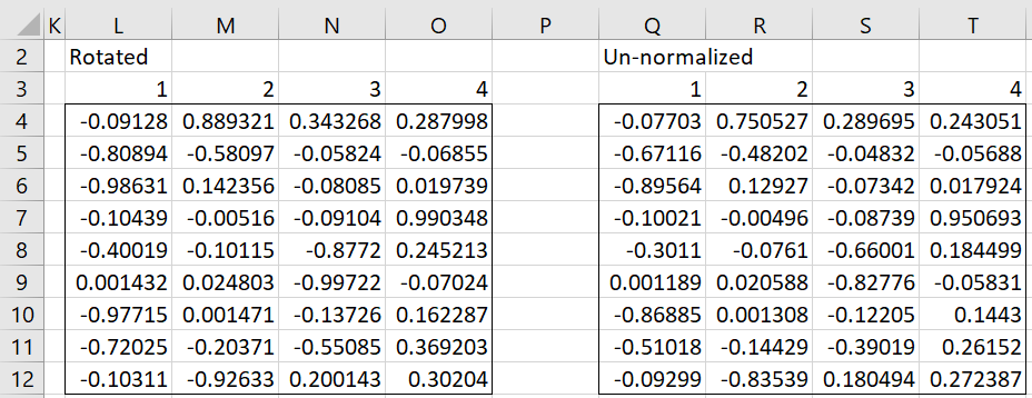
Figure 5 – Varimax final result

Here the matrix on the left (range L4:O12) is simply a copy of range A328:D336 from Figure 4. The final version of the loading factors matrix after Varimax rotation is given in range Q4:T12. For example, cell Q4 contains the formula =L4*SQRT($E4) where E4 is defined in Figure 1. Note that we can use SUMSQ(L4:O4) in place of E4 and get the same result.

Examples Workbook

Click here to download the Excel workbook with the examples described on this webpage.

References

Abdi, H. (2003) Factor rotations in Factor Analysis
https://www.utdallas.edu/~herve/Abdi-rotations-pretty.pdf

Penn State (2024) Varimax rotation
https://online.stat.psu.edu/stat505/lesson/12/12.11