Complex eigenvalues
Real Statistics Function: The Real Statistics Resource Pack provides the following function that outputs real and complex eigenvalues from a square matrix with real values.
ZEigVAL(R1, check, iter, prec): returns a 3 × n array, where n = the number of rows/columns in the square array R1. The first two rows of the output consist of the real and imaginary parts of the n eigenvalues of the square matrix A corresponding to the data in R1. Also, the third row of the output consists of the values det(A− λI) for each eigenvalue λ where I is the n × n identity matrix.
If check = TRUE (default), then the output is as described above; otherwise, only the first two rows of the output are returned.
If iter > 0 then an additional binary divide-and-conquer algorithm is applied to the real eigenvalues to improve their precision (i.e. potentially reduce the values in the last row of the output). iter = the maximum number of iterations of this algorithm (default 200).
prec is the desired precision (default .00000001). Any values whose absolute value is less than prec are treated as zero. Also, if λ = a + bi is an eigenvalue where |a| < prec, then a is replaced by 0 in the output. Similarly, if |b| < prec, then b is replaced by 0 in the output.
The order of the eigenvalues in the output is based on the following rules:
- Real eigenvalues occur to the left of complex eigenvalues
- Real eigenvalues are arranged in descending order from left to right
- Complex eigenvalues a + bi are arranged in pairs consisting of the eigenvalue with b > 0 followed immediately by its conjugate a – bi.
- Complex eigenvalues a + bi where b > 0 are arranged in descending order based on the real value a and in case of ties based on b.
Examples
Figure 1 provides two examples of the use of the ZEigVAL function. In the first example, the formula =ZEigVAL(B3:E6) shows the four eigenvalues for the 4 × 4 matrix in range B3:E6. We see that there are two real eigenvalues 6.057668 and ‑1.93994 and two complex eigenvalues 1.941134 ± .998675i.
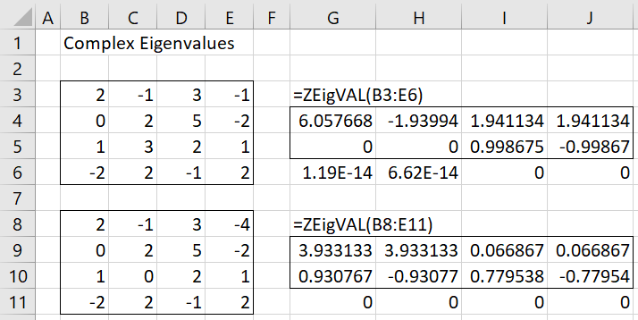
Figure 1 – Examples with complex eigenvalues
Range G6:J6 contains the values of det(A− λI) for each eigenvalue λ. We see that each of these values is near zero, as expected.
In the second example, the formula =ZEigVAL(B8:E11) produces two sets of complex eigenvalues 3.933133 ± .930767 and 0.066867 ± .779538i.
Note that the output is identical to that from the Real Statistics eigVAL function except for the order of the eigenvalues (see Eigenvalue and Eigenvector Functions).
Complex Eigenvectors
Real Statistics Function: The Real Statistics Resource Pack provides the following function that outputs real and complex eigenvalues and eigenvectors from a square matrix with real values.
ZEigVECT(R1, check, iter, prec): returns an n+4 × n+n array, where n = the number of rows/columns in the square array R1. The first row of the output consists of the eigenvalues of the square matrix A corresponding to the data in R1. Each eigenvalue is displayed in two columns: the real part followed by the imaginary part. Below each eigenvalue λ is an n × 2 range containing an eigenvector corresponding to λ.
In the second-to-last row of the output are the values det(A− λI). In the last row of the output, below each eigenvalue λ and eigenvector X is the value max {bi: i = 1 to n} where B = AX− λX.
The order of the eigenvalues and corresponding eigenvectors reading from left to right is as described for ZEigVAL. Each eigenpair consists of two columns. The first column of each eigenpair contains the real part of the eigenpair and the second column contains the imaginary part.
If check = TRUE (default), then the output is as described for ZEigVAL; otherwise, the last two rows of the output are not returned for ZEigVECT. iter and prec are as described for ZEigVAL.
All the eigenvectors output by ZEigVECT are unit eigenvectors. Note that if the eigenvalues are distinct, then the eigenvectors will be mutually independent. Repeated eigenvalues may or may not have distinct eigenvectors. Repeated eigenvalues whose eigenvectors are not distinct are called defective eigenvalues. These will result in columns of entries in the output from ZEigVECT consisting of “.” values. See Complex Eigenvalues/vectors Continued for more details.
In any case, the eigenvectors for any complex eigenvalue and its conjugate are mutually independent.
Examples
The output from =ZEigVECT(B3:E6) for the first example from Figure 1 is shown in Figure 2.
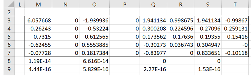
Figure 2 – Eigenvectors for the first example
Row 3 shows the same four eigenvalues shown in range G4:J5 of Figure 1 (although in a slightly different format). The corresponding eigenvectors are shown in the two columns below each eigenvalue. E.g. the eigenvector for the last eigenvalue 1.941134 – .99867i is the column vector in range S4:T7 consisting of the real values in column S and imaginary values in column T.
All the values in row 8 are near zero, which confirms that the eigenvalues are correct. All the values in row 9 are near zero, which confirms that the eigenvectors are correct.
The eigenvalues for the second example are shown in Figure 3 using the formula =ZEigVECT(B8:E11).
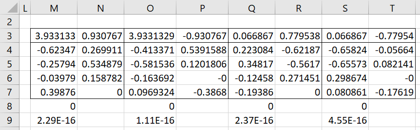
Figure 3 – Eigenvectors for two pairs of complex eigenvalues
Examples Workbook
Click here to download the Excel workbook with the examples described on this webpage.
Reference
Wikipedia (2021) Eigenvalues and eigenvectors
https://en.wikipedia.org/wiki/Eigenvalues_and_eigenvectors