Overview and Example
The Holm’s and Hochberg tests are less conservative than the Bonferroni and Dunn-Sidàk approaches in dealing with familywise error by employing stepwise adjustments to the significance level based on the rank order of the p-values of the multiple tests.
Example 1: Repeat Example 1 of Bonferroni and Dunn-Sidàk Tests using the Holm’s and Hochberg methods.
For these methods, we first rank the p-values of the k tests from smallest to largest p1 ≤ p2 ≤ … ≤ pk. We then divide the nominal significance level α by the rank to create a significance level αi = α/(k–i+1) for each test. We can do this by using Excel’s RANK.AVG function, or alternatively by sorting the p-values from smallest to largest by using Excel’s sort capability or by placing Real Statistics’ array formula =QSORTRows(A7:B12,2) in range H7:I12, as shown in Figure 1.
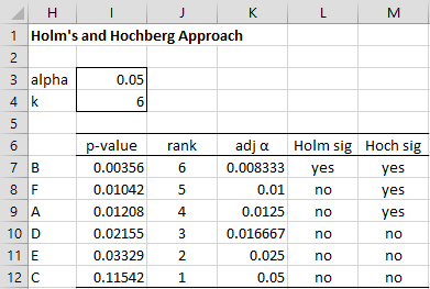
Figure 1 – Holm’s and Hochberg methods
The ranks in column J (corresponding to the values k – i + 1) go from k = 6 down to 1. The adjusted alpha values are shown in column K. E.g. cell K9 contains the formula =I$3/J9.
Holm’s Test
In Holm’s approach, we start with the smallest p-value (i = 1) and determine whether there is a significant result (i.e. p1 < α/(k–1+1) = α/k. If so we move on to the second test. We continue in this manner until we get a non-significant result (i.e. p1 ≥ α/(k–i+1)). From that point on all further tests are considered not to be significant.
In this example, p1 = .00356 < .05/6 = .008333, and so B has a significant result. Next, since p2 = .01042 < .05/5 = .01, we conclude that F has a non-significant result, as well as all the other environmental factors (A, D, E, C) below it. In Excel, we place the formula
=IF(L6=”no”,”no”,IF(I7<K7,”yes”,”no”))
in cell L7, highlight the range L7:L12 and press Ctrl-D, to get this result.
Hochberg’s Test
In the Hochberg approach, we start from the largest p-value and continue to test until we find the first significant (i.e. pi < α/(k–i+1) ) at which point all smaller pi are considered to be significant.
Since p6 = .11542 ≥ .05/1 = .05, the result for C is non-significant. Similarly, E and D have non-significant results. But p3 = .01208 < .05/4 = .0125, and so environmental factor A has a significant result. In addition, B and F, which have smaller p-values, automatically are considered to be significant. Note that F is significant even though p2 = .01042 ≥ .01.
In Excel, we get this result by placing the formula
=IF(M8=”yes”,”yes”,IF(I7<K7,”yes”,”no”))
in cell M7, highlighting the range M7:M12 and pressing Ctrl-D.
The motivation behind each of these two approaches is that once the first test step is completed then instead of k tests remaining (as in the Bonferroni correction) there are only k–1 tests remaining, and so division should be by k–1 instead of by k, and similarly for the other steps.
Observations
Hochberg’s adjustment is more powerful than Holm’s and Holm’s is more powerful (and less conservative) than Bonferroni’s (or Dunn-Sidàk’s).
Note too that we have presented the Bonferroni version of Holm’s and Hochberg’s methods; we could have used a Dunn-Sidàk version of these methods. In this case, we replace α/(k–i+1) with 1 – (1 – α) 1/(k–i+1).
Examples Workbook
Click here to download the Excel workbook with the examples described on this webpage.
Reference
Wikipedia (2018) Holm-Bonferroni method
https://en.wikipedia.org/wiki/Holm%E2%80%93Bonferroni_method
Wikipedia (2018) False discovery rate
https://en.wikipedia.org/wiki/False_discovery_rate
You can see the smoother progression.
Let’s start with this. The focus is on rank #2. My doubt is that when Hochberg has an adjusted alpha of 2.5% at rank #2, shouldn’t both test 1 and test 2 be judged at 2.5%? The familywise error formula would say, “the probability of getting a type I error on at least one of the hypothesis tests is 10%”. So, should both tests be measured at 2.5%?
Also, couldn’t the power of the test be used to override the adjusted alpha?
I have a personal adjustment to the Hochberg approach. It allows more significant results. It is calculated 2*alpha/(rank+1). In many cases, it gives the same results. In the example above though (figure 1), D and E would also be significant. The logic behind the adjustment is essentially to reduce the first influence of rank #2 to adjust alpha downward. Rank #2 for Hochberg cuts alpha in half, which is not a balanced reduction. My downward progression is .05, .033, .025, .020, .017, .014, instead Hochberg’s .05, .025, .017, .0125, .010, .008. My approach calms the initial reduction from rank #2 to .033 instead of .025. The rest of the numbers are roughly .006 to .008 apart. I have come to prefer my calculation. It’s given more interesting analyses.
What do you think?
Hi Edward,
Is there any theoretical justification for your values .05, .033, .025, .020, .017, .014 ?
Charles
The idea of this adjustment is to get a better approximation of familywise error. With Hochberg, alpha drops from 0.05 to .025 to .017. The first drop of .025 is large compared to the second drop of .008. In my method, the first drop is .017 followed by the same second drop of .008. All subsequent drops in my method are very close to Hochberg’s. So truly just the first drop from rank 1 to 2 is modified.
How does my adjustment approximate better the familywise error that increases with each test? With the formula for Familywise error, 1-(1-alpha)^c, there is a 22% chance of committing a type I error after 5 tests. Basically 1 of the tests would give a false result. The other 4 could be accepted as significant. So, if the adjusted p-value is lowered too quickly, we are tossing out valid results of significance.
Hochberg rejects half the possibly significant p-values at just rank 2. The chance of a type I error after 2 tests is roughly 10% due to familywise error (1 out of 10). Conceivably we could still accept 90% of the possibly significant p-values at rank 2. So, even an adjusted p-value of 0.45 at rank 2 could be acceptable as 10% of the possible p-values under 0.05 would not be considered significant. My approach accepts 67% of possibly significant alphas at rank 2 while Hochberg’s accepts 50%. 67% is closer to 90% than 50%. So, my adjustment looks to better approximate familywise error while still retaining some measure of protection against a false significant result.
Interesting approach. I would like to understand better the theoretical justification for your sequence versus Hochberg’s. I see that your is a smoother progression, but would others feel that it is justified?
Charles
The Benjamini-Hochberg method progresses 0.05, 0.033 then 0.017 from ranks 1 to 3 for 3 tests. In that method, the larger jump is from rank 2 to rank 3. When there are 6 tests (4 means), the second rank starts with an adjusted value of 0.041. My method is a smoother path in relation to the other methods. Sometimes my adjusted p-value is looser, sometimes it is stricter. I use my method as another method for evaluation because it is more balanced in my view. I have never used my method in a published paper though.
Hi Edward,
Your approach seems reasonable, but I don’t know whether it meets the criteria of the Holm’s and Hochberg’s tests. This would likely be necessary to use the method in a published paper.
You could check the original papers of these authors to see whether your approach would qualify.
Holm M. A simple sequentially rejective multiple test procedure. Scand J Statist 1979;6:65-70.
Hochberg Y. A sharper Bonferroni procedure for multiple tests of significance. Biometrika 1988;75:800-2. 10.1093/biomet/75.4.800
Charles