One Step of the FCS Procedure

Basic Concepts

Once all the missing data has been filled in (as described in FCS Procedure Overview) we can proceed with the FCS procedure. To do this, we start by making a better estimate of the missing data in the first column (assuming it has any missing data), then we do the same for the second column, third column, etc. until we reach the last column, after which we start all over again with the first column. We continue in this way until the specified number of iterations is reached.

Next, we show how to perform one step in this process, namely the first step where we find a better estimate for the missing data in column 1. We begin by assuming that all the cells in the first column which had missing data originally once again have missing data, but all the other columns have no missing data.

Details

For this step, we view the variable with missing data as the dependent variable y and all the other variables x₁, x₂,…, x_k as independent variables.

We consider a sample {y₁,…,y_n} of size n for the dependent variable y and samples {x_1j, x_2j,…, x_kj} for each of the independent variables x_j for j = 1, 2, …, k. We assume further that there is no missing data among the x_ij, but there may be missing data among the y_i where there are m non-missing y_i.

The following two steps are employed: a posterior step and an imputation step based on the parameters generated from the posterior step. We consider two cases: (1) where y takes a continuous set of values and (2) where the y_i are binary categorical.

We discuss the continuous variable case in the rest of this webpage. Click here for a review of the binary categorical case.

Formulas

Here we assume that y takes a continuous set of values. We start by creating a multiple regression model for Y based on the data in X using only the complete rows of X and Y (i.e. using listwise deletion). Thus, as usual

where

The posterior step now generates revised versions B′ and MS′_Res of B and MS_Res as follows:

where u is a random value from the χ²(df_Res) distribution, i.e. u = CHISQ.INV.RT(RAND(),df_Res) and

where LL^T is the Cholesky Decomposition of (X^TX)^-1 and V = [v_i] is a (k+1) × 1 column vector where each v_i is an independent random value from the standard normal distribution; i.e. each v_i = NORM.S.INV(RAND()).

Each missing data value y_i is now imputed by the value

where z_i is a random value from the standard normal distribution; i.e.

z_i = NORM.S.INV(RAND())

Note that the Cholesky decomposition of a positive definite matrix, such as (X^TX)^-1, is of form LL^T where L is a lower triangular matrix (i.e. all the values above the main diagonal are zero).

Example

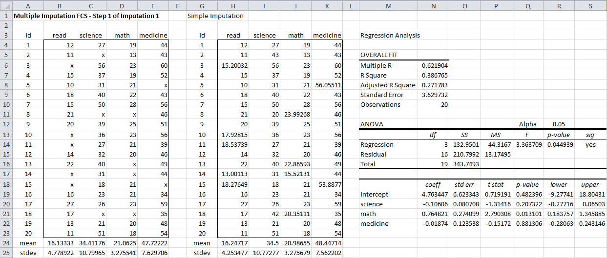
We show how this is done for the data on the left side of Figure 1, as shown in Figures 1 and 2.  

Figure 1– Simple imputation using the FCS procedure

Suppose for our original data (range B3:E23) we obtain the complete data set shown in range H3:K23 of Figure 1. We conduct a regression analysis using I3:K23 as the X input range and H3:H23 as the Y input range to obtain the results on the right side of Figure 1.

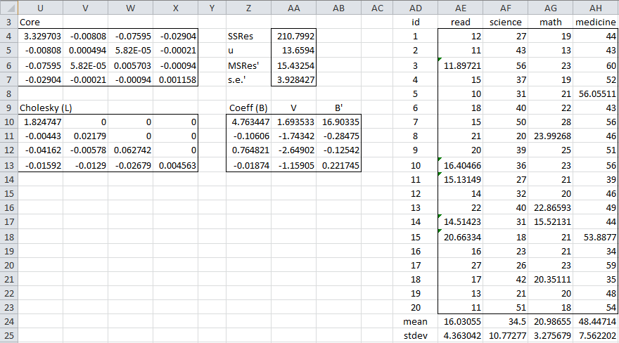
From these results, we obtain the results shown in Figure 2.

Figure 2 – Details of the FCS procedure

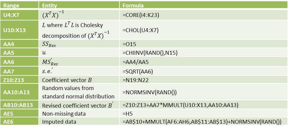
Some key formulas from Figure 2 are shown in Figure 3.

Figure 3 – Key formulas from Figure 2

Worksheet Function

Real Statistics Function: The Real Statistics Resource Pack furnishes the following array function where R1 is a range containing data in which any blank or non-numeric element is considered to be missing data and j is the number of the column that has the missing data we want to impute.

R2 is a range containing constraints and iter is the maximum number of iterations used to obtain a value within the min/max constraints (default = 25). When R2 is omitted, no constraints are used. If R2 is included then it is a 1 × 3 range that specifies constraints for column j where the column specifying the variable is not included (since it is the variable for column j).

If head is TRUE (the default) then it is assumed that the data range R1, as well as the output, contain column headings, while if head = FALSE then the R1 should not contain column headings and the output will not contain column headings either.

ImputeReg(R1, j, head, R2, iter) – generates an array where all the missing data in column j of R1 is filled in using one step of the FCS algorithm.

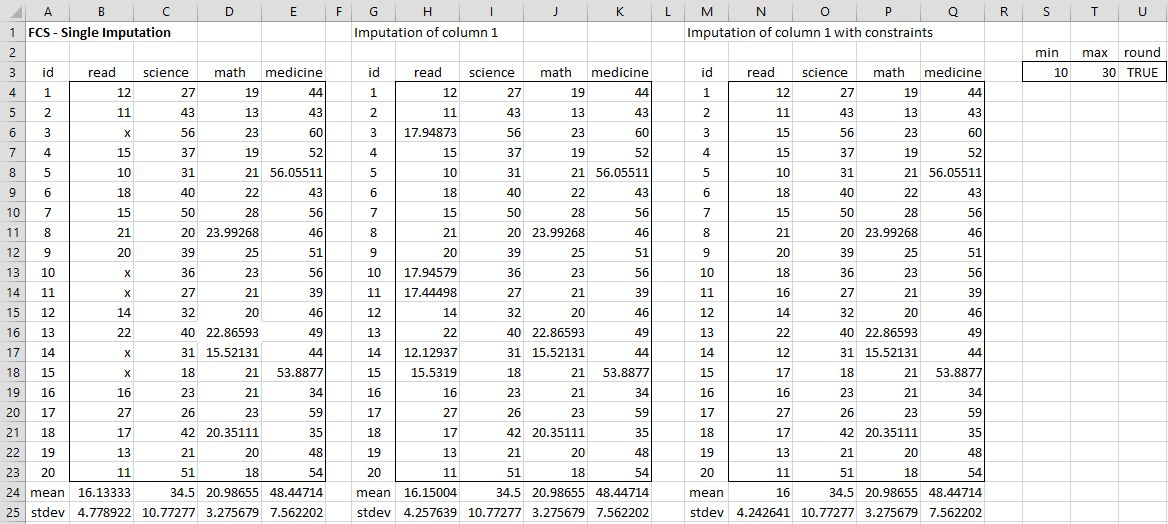
For example, in Figure 4, range H3:K23 contains the results of one iteration of the FCS algorithm on column 1 using the formula =ImputeReg(B3:E23,1). The range N3:O23 contains the results of one iteration of the FCS algorithm using the constraints specified in range S3:U3 via the formula =ImputeReg(B3:E23,1,,S3:U3).

Figure 4 – Single imputation using FCS

Examples Workbook

Click here to download the Excel workbook with the examples described on this webpage.

References

UCLA (2021) How do I perform multiple imputation using predictive mean matching in R
https://stats.oarc.ucla.edu/r/faq/how-do-i-perform-multiple-imputation-using-predictive-mean-matching-in-r/

Murray, J. S. (2018) Multiple imputation: a review of practical and theoretical findings
https://projecteuclid.org/journals/statistical-science/volume-33/issue-2/Multiple-Imputation-A-Review-of-Practical-and-Theoretical-Findings/10.1214/18-STS644.full

Woods, A. D. et al. (2021) Missing data and multiple imputation decision tree. PsyArXiv
https://doi.org/10.31234/osf.io/mdw5r

Tufis, C. (2008) Multiple imputation as a solution to the missing data problem in social sciences
https://www.revistacalitateavietii.ro/journal/article/download/538/458/883