Combining Multiple Imputations

Rubin’s combination rules

If θ is one of the parameters we are interested in and the estimates of this parameter produced by the m imputations of the missing data are θ₁, …, θ_m, with variances v₁,…, v_m, then the combined estimate of this parameter is

The within-imputation variance is then given by

and the between-imputation variance, which measures the uncertainty due to the imputation, is

The total variance is therefore

and so the standard error of the parameter is s = .

Note that the higher the value of m the lower the value of t. Note too that if there is no missing data then θ₁=⋯= θ_m and so b = 0 and t = w.

Now define the relative increase in variance due to non-response r as follows:

The test statistic for the null hypothesis θ = θ₀ is

which has a t distribution with the following degrees of freedom

With small samples an improved estimate of df′ is as follows:

where n is the sample size (complete data). This improved version of df is always less than or equal to the previous version. In fact, if the first term in the denominator of df′ is replaced by 0 we get df.

As usual, the 1 – α confidence interval for the parameter θ is expressed as

where t_crit = T.INV.2T(α/2, df).

Assumptions

The combination rules described above assume that the estimates are asymptotically normally distributed, which may not always be the case.

For example, as observed in One Sample Hypothesis Testing for Correlation Coefficient, the correlation coefficient is not normally distributed. Fortunately, as was pointed out in that webpage the Fisher transform of the correlation coefficient is normally distributed, and so we can apply the combination rules to the Fisher transform and then take the inverse transform to get a combined value for the correlation coefficient.

Worksheet Functions

Real Statistics Functions: The Real Statistics Resource Pack furnishes the following array functions where R1 is a 2m × n array where the first m rows represent the values of m imputed population parameters (mean, coefficient, etc.), and the second m rows represent the corresponding standard errors for these parameters. The columns represent separate imputations. The argument size is the number of elements in the original sample (including missing data) and lab and head are as for DescStats (where lab defaults to FALSE and head defaults to TRUE).

ImputeVar(R1, size, lab, head) – outputs an array similar to range AE15:AO19 in Figure 4 summarizing the combination rules for variance.

ImputeParam(R1, size, lab, head, alpha) – outputs an array similar to range AE23:AL27 in Figure 4 based on the combination rules and the usual t-test using the stated value of alpha (default = .05).

Example

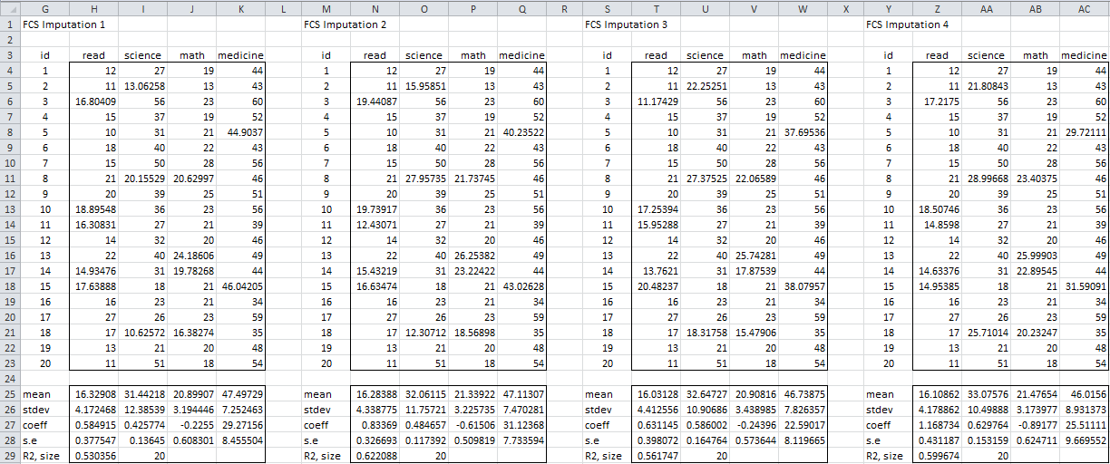
We illustrate these functions in the following figures. We begin by using ImputeFCS to generate 4 distinct imputations (see Figure 1) of the missing data in the example we have been using throughout this part of the website (see, for example, Figure 1 of Fully Conditional Specification). For each of these imputations, we use MISummary to create the compact summary described above (shown in rows 25 through 29 of Figure 1).

Figure 1 – Multiple imputations using FCS

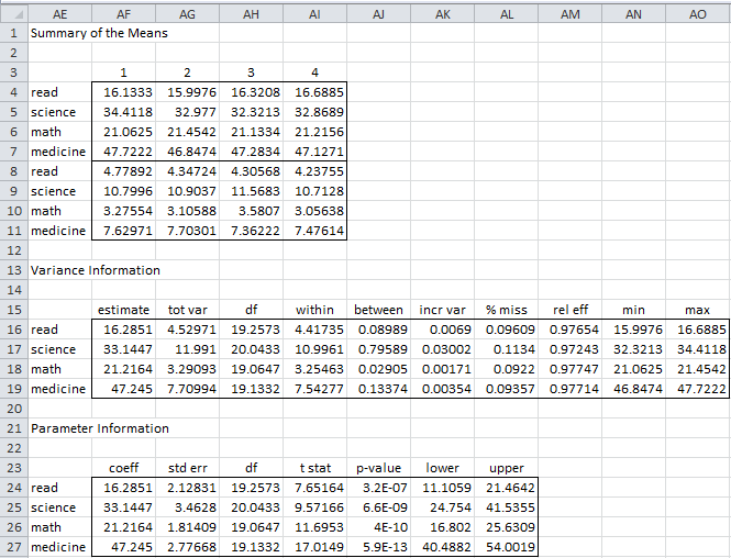
From this data, we manually create the range AE3:AI11 of Figure 2, which by way of illustration contains the means from the four imputations (in the first four rows and the standard deviations in the next four rows). The variance information (range AE15:AO19 of Figure 2) is then generated by the array formula

=ImputeVar(AE4:AI11,20,TRUE,TRUE)

The parameter information (range AE23:AL27 of Figure 2) is generated by the array formula

=ImputeParam(AE4:AI11,20,TRUE,TRUE)

Figure 2 – FCS summaries

Examples Workbook

Click here to download the Excel workbook with the examples described on this webpage.

References

Haymans, M. W., Eekhout, I (2019) Rubin’s rules. Applied missing data analysis with SPSS and (R) Studio
https://bookdown.org/mwheymans/bookmi/rubins-rules.html

UCLA (2021) How do I perform multiple imputation using predictive mean matching in R
https://stats.oarc.ucla.edu/r/faq/how-do-i-perform-multiple-imputation-using-predictive-mean-matching-in-r/

Murray, J. S. (2018) Multiple imputation: a review of practical and theoretical findings
https://projecteuclid.org/journals/statistical-science/volume-33/issue-2/Multiple-Imputation-A-Review-of-Practical-and-Theoretical-Findings/10.1214/18-STS644.full

Tufis, C. (2008) Multiple imputation as a solution to the missing data problem in social sciences
https://www.revistacalitateavietii.ro/journal/article/download/538/458/883