Table lookup functions
To illustrate Excel’s table lookup functions we use the data in Figure 1 in the examples that follow.
Figure 1 – Data range for examples
Figure 2 – Table of lookup functions
When used as an array function, =INDEX(R1, r, 0) returns the rth row from R1. Similarly, =INDEX(R1, 0, c) returns the cth column from R1. If R1 is a column vector (i.e. an r × 1 range), then =INDEX(R1, r) can be used in place of =INDEX(R1, r, 1). Similarly, if R1 is a row vector (i.e. a 1 × c range), then =INDEX(R1,,c) can be used in place of INDEX(R1,1,c).
Note that the first argument of the OFFSET function must be a reference to a single cell; it cannot be a constant or a cell range. Thus =OFFSET(4,2,3) or =OFFSET(A1:C9,2,3) would yield an error.
Details about the MATCH function
For our purposes, we only use the MATCH function when the second argument is a row or column vector. We won’t consider R taking a form such as G4:J7, only forms such as G4:J4 (row vector) or G4:G8 (column vector).
If R1 is a row range then =MATCH(x, R1, 0) returns the column number of the first incidence of x in R1. If x occurs multiple times then the column index of the first match is returned. Finally, if there is no match then #N/A is returned. You can test for such an error value by using the formula =ISERROR(MATCH(x, R1, 0)). Similarly, if R1 is a column range, then =MATCH(x, R1, 0) returns the row number of the first incidence of x in R1.
Note that when MATCH is looking for a match the formats are also matched. Thus MATCH(6,A1:E1,0) = 4 for the data in Figure 11, while MATCH(“6”,A1:E1,0) = #N/A, indicating that no match is found. The text is not case-sensitive. Thus “Z” and “z” match, as well as “cat” and “CaT”. As a result, MATCH(“z”,A4:E4,0) = 2 and not 5.
Wildcards can also be used with text: ? stands for any single character while * stands for any sequence of characters. Thus, MATCH(“?”,C1:C4,0) = 1 and not 3 since “?” is recognized as a wildcard and not the question mark character. To find the question mark you must precede the ? symbol by a tilde, and so MATCH(“~?”,C1:C4,0) = 3.
Finally, in all the previous examples, we set the third argument of MATCH to zero. Actually, this parameter can be set to -1, 0 or 1. If omitted the default value is 1.
Figure 3 – Third argument of the MATCH function
Two-dimensional table lookup
Unfortunately, the MATCH function does not give the desired result when R is a two-dimensional range. We now show various workarounds.
Suppose we would like to find the row and column numbers for the first incident of “Z” in the range A1:E4 of Figure 3. We can accomplish this as shown in the top portion of Figure 4. Here, cell L3 contains the row number of “Z” in the target range and cell L4 contains the column number of “Z” in the target range. Cells N3 and N4 display the appropriate formulas to accomplish this. Note that the first formula is an array formula while the second is not.
Figure 4 – Two-dimensional table lookup
As before, these formulas are indifferent to the case of any alphabetic character, and so if we place a small letter “z” in cell L2 the result will be the same. This approach finds the first incident of “Z” or “z” in the range A1:E1 in row precedent order (i.e. the first row is searched first, then the second row, etc.). We can easily change the two formulas to use column precedent order instead.
An alternative approach is shown in the lower half of Figure 4. This approach is only valid when the value being searched (7 in the example) occurs only once in the target range.
Finally, other approaches are described below.
Find first entry in a list
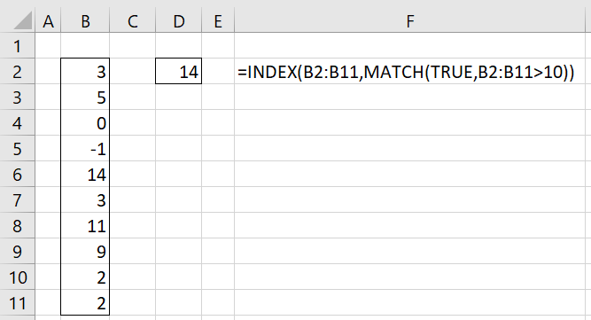
INDEX and MATCH can be used to find the first entry in a column array that exceeds a given value. E.g. you can use the array formula described in cell F2 to find the first entry in A1:A10 that exceeds 10.
Figure 5 – Finding the first entry in a list
XLOOKUP function
The following new table lookup worksheet function is available to users of Excel 2021 and 365.
XLOOKUP(x, R1, R2, not_found, match_type, search_type): looks up x in the R1 and returns the corresponding element(s) in R2.
match_type takes one of the following values when an exact match in R1 is not found:
Figure 6 – match_type
match_type = 0 is the default. A wildcard match (using * ? ~) is used when match_type = 2.
search_type takes one of the following values
Figure 7 – search_type
Figure 8 shows some examples of how to use the XLOOKUP function. The formula displayed is for the corresponding cell in column G.
Figure 8 – XLOOKUP examples
Note that we could also obtain the value in cell G25 by using the formula
=INDEX(C2:C10,MATCH(F2,A2:A10,0))
Improved two-dimensional lookup
XLOOKUP can also be used to perform lookups in two dimensions, as shown in Figure 9. The formula displayed is for the corresponding cell in column T.
Figure 9 – Two-dimensional XLOOKUP examples
Note that the value in cell T2 can also be obtained via the formula
=INDEX(M2:P5,MATCH(R2,L2:L5,0),MATCH(S2,M1:P1,0))
Examples Workbook
Click here to download the Excel workbook with the examples described on this webpage.
References
Microsoft (2021) Excel functions
https://support.microsoft.com/en-us/office/excel-functions-alphabetical-b3944572-255d-4efb-bb96-c6d90033e188#bm19
Cheusheva, S. (2022) XLOOKUP function in Excel
https://www.ablebits.com/office-addins-blog/excel-xlookup-function/
Microsoft Support (2022) XLOOKUP function
https://support.microsoft.com/en-us/office/xlookup-function-b7fd680e-6d10-43e6-84f9-88eae8bf5929


