Excel provides the INDEX, MATCH and OFFSET functions that can be used for table lookup. See Table Lookup Functions for more details. On this webpage, we give four examples describing how to use these functions for table lookup.
We also describe how to use interpolation when performing table lookup.
Excel Examples
Equally spaced numeric headings
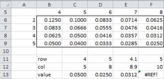
Example 1: Create a way of finding the value in the following table for any row and column heading.
Figure 1 – Table lookup for equally spaced headings
For any row heading r and column heading c, the table value is INDEX(R1, r – 1, c – 3) where R1 is the array where the table is stored (i.e. B6:F9 in Figure 1). The argument r – 1 is simply r – r1 + 1 where r1 is the first-row heading (2 in this example). Similarly c – 3 is c – c1 + 1 where c1 = 4, the first column heading.
E.g., the table value where r = 4 and c = 5 is 0.0500 as shown in cell C13 in Figure 1. This is accomplished using the formula =INDEX(B6:F9, C11–A6+1, C12–B5+1).
This approach only works where headings are equally spaced (i.e. interval data). With this approach, decimal values of r or c are equivalent to INT(r) and INT(c). If r and/or c are out of range then an error is generated. For this example, this occurs if r < 2, r ≥ 5, c < 4 or c ≥ 9.
Any headings
Example 2: Create a way of finding the value in the following table for any row and column heading

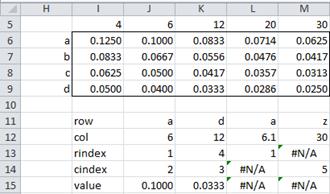
Figure 2 – Table lookup for any type of headings
This time we will look for an exact match of the row or column heading. For a given row value r and column value c, we first find the row and column index to the table. The row index is MATCH(r, R1, 0) and the column index is MATCH(c, R1, 0) where R1 is the array where the table is stored.
The 3rd argument of 0 indicates that only an exact match is acceptable. The row index of a is 1 (since the heading of the first row is a). Similarly, the column index of 6 is 2 (since the heading of the second column is 6). The table value is then INDEX(R1, row-index, col-index), i.e. INDEX(R1, 1, 2) in this example.
E.g., the table value where r = “a” and c = 6 is 0.1000 as shown in cell J15 in Figure 2. We accomplish this using the formula =INDEX(I6:M9, J13, J14). Here cell J13 contains the formula =MATCH(J11, H6:H9, 0) and cell J14 contains the formula =MATCH(J12, I5:M5, 0).
Unless there is an exact match an error is returned.
Using interpolation
Example 3: Create a way of finding the value in the following table for any row and column heading.
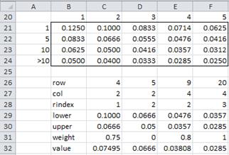
Figure 3 – Table lookup for headings in intervals
The row headings define four ranges: 1-4, 5-9, 10 and more than 10. For a given row value r and column value c, we first find the row and column index to the table. The column index is simply the column heading. We use MATCH(r, R1) as the row index, where R1 is the array where the table is stored. This is similar to the approach used in Example 2, except that this time we are not looking for an exact match. We now look up the table entry corresponding to r and c (i.e. the lower value) as well as the table entry corresponding to r + 1 and c (the upper value).
The result we are looking for is an interpolation between these two values. In order to carry out this interpolation, we calculate a weight, which is a value between 0 and 1. Weights close to 0 favor the lower value and weights close to 1 favor the upper value. We use Excel’s OFFSET function to calculate the value of these weights.
E.g., the table value where r = 4 and c = 2 is 0.07495 as shown in cell C32 in Figure 3. This is accomplished using the following formulas:
 Figure 4 – Some formulas from Figure 3
Multiple tables
Example 4: Create a way of finding the value in the following tables for any row and column heading and value of α.
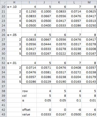
Figure 5 – Table lookup with multiple tables
Here we have three tables like those in Example 1. The first table corresponds to a value of α = .10, the second to α = .05 and the third to α = .01. The approach is the same as in Example 1, except that we need to account for all three tables. One approach is to assume that the table corresponding to α = .05 is the base table and use an offset of 6 rows forward or back to get to the other two tables. The number 6 is simply the number of rows in the Excel worksheet between any cell in the second table and the corresponding cell in the first or third table.
We can use the Excel function OFFSET(R1, c, 0) which refers to the range R1 offset by c rows and 0 columns. When c = 6 this refers to the third table, when c = -6 this refers to the first table and when c = 0 this refers to the second table.
E.g., the table value where r = 4, c = 5 and α = .01 is 0.0500 as shown in cell L43 in Figure 5. This is accomplished using the formula
=INDEX(OFFSET(I27:M36, L42, 0), L38–H27+1, L39–I26+1)
where cell L42 contains the formula =IF(L40=0.01,6,IF(L40=0.1,-6,0)).
Worksheet Functions
Real Statistics Functions: Since some of the table lookup approaches described above can be somewhat complex, the Real Statistics Pack provides the following useful table lookup functions:
MLookup(R1, r, c) = returns the value in the table defined by range R1 in the row headed by r and the column headed by c. Here R1 includes both the data and row/column headings.
ILookup(R1, r, c) = returns the value in the table defined by range R1 corresponding to row r and column c. If r or c can refer to some value that must be interpolated between row or column headings, provided those headings are numbers. If the first row (or column) heading is preceded by “>” it refers to values smaller than the next row (or column heading). If the last row (or column) heading is preceded by “>” it refers to values bigger than the previous row (or column heading). Here R1 includes both the data and row/column headings.
MLookup (match table lookup) implements the method in Example 2. Thus the table value where r = “a” and c = 6 is 0.1000 as shown in cell J15 in Figure 2 can be provided using the formula =MLookup(H5:M9, J11, J12).
ILookup (interval table lookup) implements the method in Example 3. Thus the table value where r = 4 and c = 2 is 0.075 as shown in cell C32 in Figure 3 can be provided by the formula =ILookup(A20:F24, C26, C27). Similarly, the value where r = 20 and c = 4 is as shown in cell F32 can be provided by the formula =ILookup(A20:F24, F26, F27).
Interpolation
Related to ILookup is the interpolation function:
INTERPOLATE(r, r1, r2, v1, v2, h) = returns the value between v1 and v2 that are proportional to the distance that r is between r1 and r2, where v1 corresponds to r1 and v2 corresponds to r2.
INTERPOLATE(r, r1, r2, v1, v2, 0) = v1 + . For example, INTERPOLATE(3, 2, 6, 10, 30, 0) = 15 since 3 is one-fourth the way between 2 and 6 and 15 is one-fourth the way between 10 and 30.
When h = 0, then linear interpolation is used as described above. If h = 1 (default) then harmonic interpolation is used, as described at Interpolation.
Examples Workbook
Click here to download the Excel workbook with the examples described on this webpage.
References
Microsoft (2021) Excel functions
https://support.microsoft.com/en-us/office/excel-functions-alphabetical-b3944572-255d-4efb-bb96-c6d90033e188#bm19
Microsoft (2012) MATCH function
https://support.microsoft.com/en-us/office/match-function-e8dffd45-c762-47d6-bf89-533f4a37673a
Microsoft (2012) INDEX function
https://support.microsoft.com/en-us/office/index-function-a5dcf0dd-996d-40a4-a822-b56b061328bd
Microsoft (2012) OFFSET function
https://support.microsoft.com/en-us/office/offset-function-c8de19ae-dd79-4b9b-a14e-b4d906d11b66
Wikipedia (2025) Interpolation
https://en.wikipedia.org/wiki/Interpolation


In Example 4, how would you find the data points that need to be interpolated between the tables. For example if alpha=0.03? As well as among the rows and columns if r=4.5 and c=3.2?
Alexis,
Let’s first consider the case where you have table values for positive integer values of r and c and alpha = .03. In fact, let’s suppose that the values for alpha = .03 are as in the following table:
r..c..value
4..3..10
4..4..20
5..3..30
5..4..50
Interpolating first for r, we find the following values
r….c..value
4.5..3..20
4.5..4..35
Now we need to interpolate on c to get 20+(35-20)*.2 = 23.
If there is not table value for alpha = .03, but there are table values for alpha = .02 and .05, then you repeat the above process to get a value where r = 4.5, c = 3.2 and alpha = .02. You also repeat this process to get a value for r = 4.5, c = 3.2 and alpha = .05. Finally, you perform interpolation on alpha between these values.
The above shows how to perform linear interpolation. You can perform harmonic interpolation in a similar manner.
Charles